6  Air pollution module

6.1 Executive summary

Policies aimed to reduce GHG emissions, such as carbon pricing, can lead to a reduction in ambient air pollution, a major health risk¹, due to the co-emission of GHGs and local pollutants when burning fossil fuels. Local pollutants, such as BC, OC, NH₃, SO₂ and NMVOC are responsible for the formation of fine particulate matter (PM_2.5) and ozone (O₃) pollution, with known health impacts. CPAT quantifies reductions in mortality and morbidity from improved air quality as part of the co-benefits of carbon pricing.

The air pollution module in CPAT is mostly based on models developed by external institutions and researchers, but also includes modeling developed specifically for CPAT. The main inputs are: (1) energy consumption in time and scenario by fuel type and sector from the Mitigation module, (2) emission factors net of projected average use of pollution control equipment, fuel processing and combustion method from GAINS model², (3) concentrations of PM_2.5 and ozone for the baseline year, (4) emissions-to-concentrations relationships based on source receptor matrices (TM5-FASST), regression analysis, machine learning models, source apportionment studies and intake fractions, (5) relative risk functions³ for exposure to PM_2.5 and O₃, and (6) population projections in time.

The main results from the air pollution module are mortality and disability adjusted life-years (DALYs) attributed to air pollution (ambient and household) under the baseline and the carbon price scenario. Other outputs include: (1) the economic valuation of averted deaths (using a transferred value of the statistical life), (2) health expenditure, (3) working days lost due to pollution, and (4) market output losses due to morbidity and mortality.

Reduced-form approximations are used to estimate emissions, concentration of pollutants and health effects. We use and adapt the results of more complex models into simplified relationships. For instance, in the case of the relationship between emissions of pollutants and ambient concentrations of PM_2.5 and ozone, CPAT includes the option to use the results from a linear emulator of a complex global chemical transport model. The results of the air pollution module are in line with other more complex models (see Section 6.8), although both CPAT and the models to which we compare to are subject to uncertainty and the results may be sensitive to the assumptions used. We address this issue in CPAT by allowing the user to input local information, if available, and to switch among methodological options (with the best options possibly dependent on the country chosen).

Caveats in the air pollution module include the use of international databases, the country level (instead of sub national) and annual resolution of the analysis and the uncertainty on estimations. Section 6.9 provides some insights on how the user can tackle these caveats.

6.2 List of Acronyms

Institutions

IHME Institute for Health Metrics and Evaluation

IIASA International Institute for Applied Systems Analysis

ILO International Labour Organization

IMF International Monetary Fund

IPCC The Intergovernmental Panel on Climate Change

OECD Organization for Economic Co-operation and Development

WHO World Health Organization

Abbreviations

BoD Burden of Disease

CPAT Climate Policy Assessment Tool

CLE Current Legislation Scenario

CPI Consumer Price Index

DALY Disability-adjusted life year

EDGAR Emissions Database for Global Atmospheric Research

EF Emission Factor

FASST Fast Scenario Screening Tool

GAINS Greenhouse Gas - Air Pollution Interactions and Synergies

GBD Global Burden of Disease

GDP Gross Domestic Product

GEPR Getting Energy Prices Right

GHED Global Health Expenditure Database, WHO

GTP Global Temperature Potential

GWP Global Warming Potential

HAP Household air pollution

IER Integrated Exposure Response

LPG Liquified Petroleum Gas

OAP Outdoors air pollution

PAF Population Attributable Fraction

PPP Purchasing Power Parity

PTB Preterm birth

RR Relative Risk

SLCF Short-lived climate forcers

THE Total Health Expenditure

TMREL Theoretical minimum risk exposure level

UNFCCC United Nations Framework Convention on Climate Change

VSL Value of the statistical life

YLL Years of life lost

Pollutants and substances

BC Black Carbon

CH4 Methane

CO Carbon monoxide

HFCs Hydrofluorocarbons

NF3 Nitrogen triflouride

NMVOC Non methanic volatile organic compounds

NOx Nitrogen oxides

O3 Ozone

OC Organic Carbon

PFCs Perfluorocarbons

PM_2.5 Particulate matter (PM) that have a diameter of less than 2.5 micrometers

POM Primary Organic Matter

SF6 Sulphur hexafluoride

SO2 Sulfur dioxide

Units

6mDMA8h Six-month period with the highest mean, 8-h daily maximum concentration metric

GJ Giga Jules (1 GJ =10^9 jules)

µg/m3 Micrograms per cubic meter

ktoe kilotons of oil equivalent

PJ Peta Jules (10^15 Jules)

ppb parts per billion

6.3 Introduction

The present Chapter focuses on the methodology followed in CPAT to assess the air pollution development co-benefits of carbon pricing.

Figure 6.1 shows an overview of the methodology, where the red box highlights the topics covered in this document. As presented in the figure, the air pollution tab receives as an input the energy consumption for the different sectors and fuels from the Mitigation tab. Emissions (of local and global pollutants) are calculated in the Mitigation tab of CPAT, but the data sources and methodology used is covered in this Chapter. Based on emissions estimates, the Air Pollution tab calculates for each year the concentration of PM_2.5 and O₃, the health impacts attributed to pollution (deaths and DALYs) and economic impacts of pollution.

Figure 6.1: Overview of CPAT methodology

The health impacts attributable to air pollution methodology is presented in Figure 6.2. As shown in the figure, the total health burden of pollution is estimated for the baseline scenario and for the carbon price scenario. The impact of the carbon price is then estimated as the difference between the total burden under both scenarios.

Figure 6.2: Methodology for estimating health impacts of a carbon price

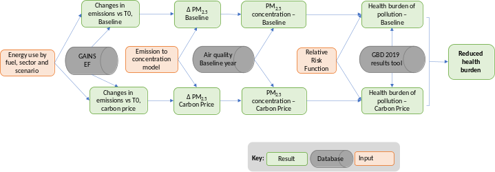
The methodological steps presented in Figure 6.1 and Figure 6.2 are described in the following sections. Section 6.4 presents the sources and methods for estimating emissions. Section 6.5 explains the relationship between emissions and ambient pollution. Section 6.6 introduces the quantification of the health burden of air pollution and Section 6.7 presents the quantification of the economic impacts of pollution. This Chapter presents additional sections to validate findings (Section 6.8) and make the user aware of the limits (Section 6.9) of the air pollution module.

6.4 Methods for calculating emissions

In this section we explain how we calculate emissions in CPAT (Mitigation tab), using as input the fuel consumption by sector and over time, and emission factors (Figure 6.3). Emissions will be used to calculate concentrations of PM_2.5 and O₃.

Figure 6.3: Overview of CPAT methodology, highlighting Emissions

6.4.1 Data sources for emissions

Input	Source
Energy consumption by fuel and sector in time	CPAT mitigation module. Based in IEA energy balances (IEA 2019) and others. See Mitigation tab documentation.
Emission Factors	GAINS model, IIASA (Wagner et al. (2020))
Radiative coefficients	GAINS model, IIASA (Wagner et al. (2020))

6.4.2 Emission factors from GAINS

Emissions for the baseline scenario are taken from the Greenhouse Gas - Air Pollution Interactions and Synergies (GAINS) Global Model, from the International Institute for Applied Systems Analysis (IIASA). The GAINS scenario selected as baseline is the ECLIPSE_V5a_CLE_base. This dataset was created in June 2015 and it covers emissions from 1990 to 2050 in five-year intervals. This baseline scenario considers current legislation (CLE) and committed legislation. The emission factors were grouped to reflect CPAT sectors and fuels, as described in Wagner et al. (2020).

The basic principle to estimate emissions in GAINS is presented in expression (Equation 6.1). Emissions are driven by activity levels (such as energy consumption), emissions factors that depend on the process and fuel type utilized (if any) and technology implementations that account for possible pollution control technologies (such as particulate filters, electrostatic precipitators, among many others). The emission factors used in CPAT include country specific technology implementations, according to the Current Legislation Scenario.

\[Emissions = FuelConsumption*Emission\ Factors \tag{6.1}\]

In CPAT, the pollutants included are PM_2.5, NOx, SO₂, CO₂, NMVOC, BC, OC, CH₄, CO, while the sectors and fuels for which we have emissions factors are presented in Table 6.1 ⁴.

Table 6.1: Emission factor sectors and fuels

Sector	Subsector	Biomass	Coal	Diesel	Gasoline	Jet fuel	Kerosene	LPG	Natural Gas	Other oil products
Power		X	X	X	X				X	X
Residential		X	X	X	X		X	X	X	X
Transport	Road transport			X	X		X	X	X
	Aviation					X
	Rail			X
Industries	Construction			X	X		X	X	X
	Food and Forestry	X	X	X	X		X	X	X	X
	Mining & Chemicals			X	X				X
	Manufacturing	X	X	X	X		X	X	X	X
	Other Manufacturing	X	X	X	X		X	X	X	X
	Services	X	X	X	X		X	X	X	X

Source: Own elaboration based on Wagner et al. (2020)

The EF from the current legislation scenario will change in time, as shown in Figure 6.4. In CPAT, the user can select the to use EFs that are variable in time or a constant value, from year 2015.

Figure 6.4: Example of emission factors for SO₂, for power plants in India

Source: Own elaboration based on Wagner et al. (2020)

The EF from GAINS are country specific for 89 countries. For countries not included in that group, we consider regional averages.

Figure 6.5 shows data quality categories for countries included in the GAINS model. In green is Category 1, for which there is high confidence in the data. In yellow is category 2, for which there is medium confidence and in red, is category 3, for which the level of confidence is low.

Figure 6.5: Quality of input data. Data quality categories (QC)

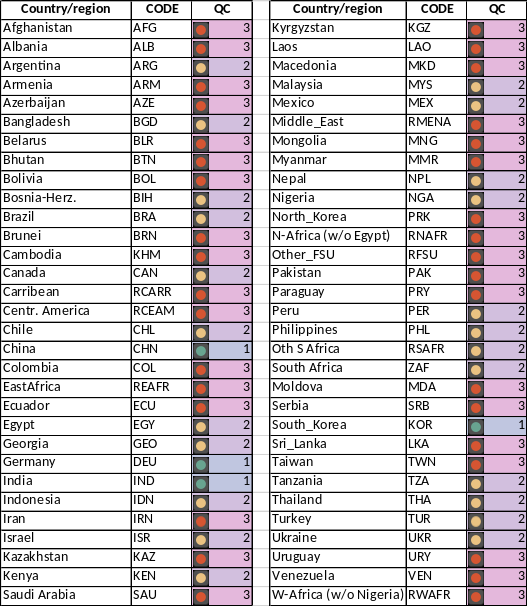
Source: Personal communication with Fabian Wagner. Category 1: High confidence, Category 2: Medium confidence Category 3: Low confidence.

6.4.3 Radiative forcing coefficients

Reducing local air pollutants will result in positive health impacts. However, the reduction of local pollutants can imply an increase in global warming, because of the cooling effect of some of these pollutants. Some local pollutants behave asymmetrically compared to GHGs: the more they are emitted, the more they cool the earth. Figure 6.6 presents a diagram of the cooling and warming effects of reducing pollutants.

Figure 6.6: Diagram of the impact of pollution control on emissions and climate impact

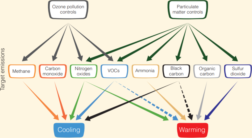
Source: Shindell (2013)⁵. Solid lines indicate known impact; dashed lines indicate uncertain impact.

CPAT will consider the net warming effects of reducing local pollutants, according to their Global Warming Potential in a hundred years (GWP100), using the regional values presented in Table 6.2.

Table 6.2: GWP100 coefficients used in CPAT

Region	CO	NH3	NOx	PM_BC	PM_OC	SO2	VOC
Africa	1.989	-13.332	-7.058	356.463	-121.075	-85.172	6.154
Asia & Oceania	1.989	-13.332	-7.058	356.463	-121.075	-85.172	6.154
Eurasia	3.246	-18.162	-9.501	407.156	-138.559	-109.67	7.303
Europe	3.246	-18.162	-9.501	407.156	-138.559	-109.67	7.303
Middle East	1.989	-13.332	-7.058	356.463	-121.075	-85.172	6.154
North America	1.989	-13.332	-7.058	356.463	-121.075	-85.172	6.154

Source: GAINS model, IIASA.

Besides CO₂ emissions, CPAT will consider the Global Warming Potential of methane, using the GWP100 indicated in Table 6.3.

Table 6.3: GWP100 coefficients for CH4 used in CPAT

Substance	GWP100	Source
CH4	28.0	IPCC 5th assessment report

Source: IPCC and others (2014).

A list of substances with radioactive forcing impacts is presented in Table 6.4. The table indicates which substances are included in CPAT and in the UNFCCC framework.

Table 6.4: Substances with climate/radiative forcing impacts under UNFCCC and CPAT

Substance type	Substance	UNFCCC	CPAT
Greenhouse gases	CO2	✓	✓
	CH4	✓	✓
	N2O	✓	✕
	HFCs	✓	✕
	PFCs	✓	✕
	SF6	✓	✕
	NF3	✓	✕
Short-lived climate forcers (SLCF)	BC	✕	✓
	O3 (tropospheric)	✕	✕*
	CH4	✓	✓
	HFCs	✓	✕
	SO2	✕	✓
	NOx	✕	✓
Precursors of SLCF	CO	✕	✓
	NMVOC	✕	✓
	SO2	✕	✓
	NOx	✕	✓
	NH3	✕	✕
	OC	✕	✓

Source: Own elaboration. (*) CPAT includes the health effects of ambient ozone, but not emissions of ozone.

6.5 Methods to relate emissions and ambient pollution

This chapter describes the options implemented in CPAT to link emissions and ambient pollution: i) TM5-FASST model, ii) Source apportionment information combined with FASST, iii) Elastic Net model, iv) Intake fractions, and v) Machine learning (see Figure 6.7).

Figure 6.7: Concentration of PM_2.5 and O3, CPAT methodology overview

Table 6.5 describes the aggregation of sectors done in the air pollution tab, which in some cases differs from the sector used in the Mitigation tab.

Table 6.5: Source types in the Air pollution and Mitigation modules

Air pollution aggrupation	Air pollution Subsector code	Manufacturing sub sectors	Mitigation sub sectors	Fuel used
Coal Power Plants	pow		Power	coa
Gas Power Plants				nga
Other Power Plants				oop
				bio
Road transport	rod		Road	multiple
Residential, services and construction	res		Residential	multiple
	cst		Construction	multiple
	srv		Services	multiple
Industries and other energy	mnf	irn	Iron and steel	multiple
		nfm	Non-ferrous metals	multiple
		mac	Machinery	multiple
		cem	Cement	multiple
		ftr	Fuel transformation & transportation	multiple
	mch		Mining & Chemicals	coa
	omn		Other manufacturing	coa
	oen		Other - energy use	multiple
	ral		Rail	die
	avi		Domestic Aviation*	jfu
Food & forestry	foo		Food & forestry (includes agriculture)	multiple

Source: Own elaboration. (*) considers emissions from departing and landing only.

6.5.1 Data sources to relate emissions and ambient concentrations

Table 6.6: Summary of data sources to relate emissions to ambient pollution

Input	Source
TM5-FASST model, from the European Commission Joint Research Center	Van Dingenen et al. (2018)
TM5-FASST mode, downscaled at a country level	Aleluia Reis (2020)
Elastic Net Model & Machine learning models	Renna and Reis (2021)
WHO source apportionment database	World Health Organization (2015)
Other source apportionment studies	World Bank (2020); World Bank (2019a) Lelieveld et al. (2015); Almeida et al. (2020); Gaita et al. (2014)
Intake fractions	Zhou et al. (2006); Apte et al. (2012)

6.5.2 Option 1: TM5-FASST

The Fast Scenario Screening Tool (FASST) is an emulator of the full TM5-CTM global chemical transport model. FASST is a source-receptor model with linearized relations between emissions and concentrations. This tool allows the modeling of ambient PM_2.5 and O₃ concentrations.

FASST includes 56 source-receptor regions (see Figure 6.8) and the pollutants considered (as emissions) are SO₂, NOx, NH₃, OC, NMVOC, Elemental Carbon, Primary Organic Matter⁶, PM_2.5⁷ and CH₄.

Figure 6.8: The 56 continental emission source regions in TM5-FASST

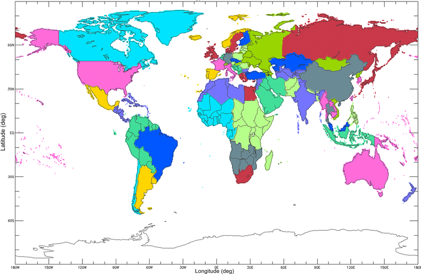
Source: Van Dingenen et al. (2018)

The coefficients from the source-receptor matrices are given by Equation 6.2 and the concentration in receptor \(y\) from component \(j\) are presented in Equation 6.3 - see Van Dingenen et al. (2018).

\[A_{\text{ij}}\left\lbrack x,\ y \right\rbrack = \frac{\mathrm{\Delta}C_{j}(y)}{\mathrm{\Delta}E_{i}\left( x \right)} \tag{6.2}\]

With \(\mathrm{\Delta}E_{i}\left( x \right) = 0.2E_{i,base}\left( x \right)\)

Where:

\(A_{\text{ij}}\): source-receptor matrix coefficient (annual mean responses) in \(\mu\)g/m3

\(x\): source region

\(y\): receptor point

\(j\): component (PM_2.5 and O₃)

\(i\): precursor of j (BC, POM, SO2, NOx and OPM for j = PM2.5; and NOx, NMVOC, SO2 and CH4 for j= O3)

Ambient concentration in receptor \(y\) from component \(j\) is calculated using expression (Equation 6.3).

\[C_{j}\left( y \right) = C_{j,\ base}\left( y \right) + \sum_{k = 1}^{n_{x}}{\sum_{i = 1}^{n_{i}}{A_{\text{ij}}\left\lbrack x_{k},\ y \right\rbrack*\left\lbrack E_{i}\left( x_{k} \right) - E_{i,\ base}\left( x_{k} \right) \right\rbrack*UrbanIncFactor}} \tag{6.3}\]

Where:

\(A_{\text{ij}}\): source-receptor matrix coefficient (annual mean responses)

\(n_{i}\): number of precursors \(i\)

\(n_{x}\): number of source regions \(x\)

\(E_{i}(x)\): emission rate (kg/yr) of precursor I at source x

\(C_{j,\ base}\left( y \right)\): constant for pollutant \(j\) and location \(y\)

\(k\): pollutant

The precursors for PM_2.5 included are BC, POM, SO2, NOx and OPM (other particulate matter). Notice that NH3 emissions are not included in the analysis and are assumed to be constant over time.

The precursors of ozone considered are NOx, NMVOC, SO2 and CH4.

As mentioned, FASST contains results for 56 regions only. To produce source-receptor coefficients for every country inside those regions, we applied a down-scaling of FASST to produce country level coefficients. The methods are described in Aleluia Reis (2020).

In addition to the country down-scaling from Aleluia Reis (2020), we produced a downscale based in the population in the FASST regions and in the countries inside those regions, as presented in expression Equation 6.4. In some cases, we applied the population downscale, when the performance of the method described in Aleluia Reis (2020) is low.

\[A_{i,j,country} = A_{i,j,region}*\frac{\text{Population}_{\text{region}}}{\text{Population}_{\text{country}}} \tag{6.4}\]

If we multiply the emissions \(j\) from the modeled sectors by the corresponding \(A_{i,j}\) coefficients, we obtain the `modeled’ contribution to \(i\)(where \(i\) is PM_2.5 or O3) in CPAT, using expression Equation 6.5.

\[\text{Modeled\ }i_{t,s} = \sum_{j}^{}{\sum_{s}^{}{A_{i,j}*Emissions_{j,s,t}}} \tag{6.5}\]

6.5.2.1 From FASST spreadsheet to CPAT

In the spreadsheet version of FASST (provided by Rita Van Dingenen), there are two emission scenarios and each of them is compared to FASST baseline scenario (there are three scenarios in total). In CPAT, we do not use the FASST baseline scenario, but only two scenarios: baseline (as in CPAT) and carbon price (as in CPAT). We do not need to include the FASST baseline scenario in CPAT because to quantify the changes in PM_2.5 (or in O3), attributed to the carbon tax, we subtract the results from the baseline and the carbon tax. In that operation, FASST baseline would be eliminated anyways and because of that is not needed.

Table 6.7 presents the operations in FASST spreadsheet and CPAT adaptations. In the last column of the table, I mention the ‘transformations’ to the SR coefficients used in CPAT, so the operations are simplified. These transformations yield the same changes in PM_2.5 that we would obtain using the original steps performed in the spreadsheet of FASST, because all operations are linear.

Table 6.7: CPAT adaptations of TM5-FASST, spreadsheet version

Emissions	FASST spreadsheet calculation (USER_CALC_1)	CPAT adaptations
Uses BC emissions	\(\text{delta}_{BC - > BC,1} = \left( Em_{BC,1} - EmFASST_{\text{BC}} \right)*SR_{BC - > BC}\)	In CPAT I multiply BC emissions by \(SR_{BC - > BC}*urbanIncfactor = \mathbf{S}\mathbf{R}_{\mathbf{BC,\ CPAT}}\)
Uses POM emissions= 1.3*OC	\(\text{delta}_{POM - > POM} = \left( Em_{POM,1} - EmFASST_{\text{POM}} \right)*SR_{POM - > POM}\)	In CPAT I multiply POM emissions by \(SR_{POM - > POM}*urbanIncfactor = \mathbf{S}\mathbf{R}_{\mathbf{POM,\ CPAT}}\)
Uses Other PM emissions = PM2.5-BC-POM	\(\text{delta}_{OPrPM2.5 - > OPrPM2.5,1} = \left( Em_{OPrPM2.5,1} - EmFASST_{OPrPM2.5} \right)*SR_{\mathbf{BC - > BC}}\)	In CPAT I multiply Other PM2.5 emissions by \(SR_{BC - > BC}*urbanIncfactor = \mathbf{S}\mathbf{R}_{\mathbf{BC,\ CPAT}}\)
Uses SO2 emissions	\(\text{delta}_{SO2 - > SO4,1} = \left( Em_{SO2,1} - EmFASST_{SO2} \right)*SR_{SO2 - > SO4}\)	In CPAT, I multiply the emissions of SO2 by \(SR_{SO2 - > SO4} + \ SR_{SO2 - > NO3} + \ SR_{SO2 - > NH4} = \mathbf{S}\mathbf{R}_{\mathbf{SO2,\ CPAT}}\)
	\(\text{delta}_{SO2 - > NO3,1} = \left( Em_{SO2,1} - EmFASST_{SO2} \right)*SR_{SO2 - > NO3}\)
	\(\text{delta}_{SO2 - > NH4,1} = \left( Em_{SO2,1} - EmFASST_{SO2} \right)*SR_{SO2 - > NH4}\)
Uses NOx emissions	\(\text{delta}_{NOx - > SO4,1} = \left( Em_{NOx,1} - EmFASST_{\text{NOx}} \right)*SR_{NOx - > SO4}\)	In CPAT, I multiply the emissions of NOx by \(SR_{NOx - > SO4} + \ SR_{NOx - > NO3} + \ SR_{NOx - > NH4} = \mathbf{S}\mathbf{R}_{\mathbf{NOx,\ CPAT}}\)
	\(\text{delta}_{NOx - > NO3,1} = \left( Em_{NOx,1} - EmFASST_{\text{NOx}} \right)*SR_{NOx - > NO3}\)
	\(\text{delta}_{NOx - > NH4,1} = \left( Em_{NOx,1} - EmFASST_{\text{NOx}} \right)*SR_{NOx - > NH4}\)
Uses NH3 emissions	\(\text{delta}_{NH3 - SO4,1} = \left( Em_{NH3,1} - EmFASST_{NH3} \right)*SR_{NH3 - SO4}\)	In CPAT, we do not have NH3 emissions
	\(\text{delta}_{NH3 - > NO3,1} = \left( Em_{NH3,1} - EmFASST_{NH3} \right)*SR_{NH3 - > NO3}\)
	\(\text{delta}_{NH3 - > NH4,1} = \left( Em_{NH3,1} - EmFASST_{NH3} \right)*SR_{NH3 - > NH4}\)

Where \(\text{EmFASST}\) are FASST base emissions and \(Em_{p,1}\) are emissions from pollutant \(p\) in scenario 1.

In the tab USER_CALC_1, \(\text{delta}_{\text{BC}}\) and \(\text{delta}_{\text{POM}}\) are then multiplied by the urban incremental factor.

\[d_{BC,1} = delta_{BC,1}*urbIncfactor \tag{6.6}\]

\[d_{POM,2} = delta_{POM,1}*urbIncfactor \tag{6.7}\]

And the following aggregations among deltas are made:

\[d_{SO4,1} = delta_{SO2 \rightarrow SO4,1} + delta_{NOx - > SO4,1} + delta_{NH3 - SO4,1} \tag{6.8}\] \[d_{NO3,1} = delta_{SO2 - > NO3,1} + delta_{NOX - > NO3,1} + delta_{NH3 - > NO3,1} \tag{6.9}\]
\[d_{NH4,1} = delta_{SO2 - > NH4,1} + delta_{NOx - > NH4,1} + delta_{NH3 - > NH4,1} \tag{6.10}\]
\[d_{OPrPM2.5,1} = delta_{OPrPM2.5 - > OPrPM2.5,1} \tag{6.11}\]

Finally, the total change in PM_2.5 concentrations in scenario 1 is:

\[\text{TOTdP}M_{1} = d_{BC,\ 1} + d_{POM,\ 1\ } + d_{SO4,1} + d_{NO3,1} + d_{NH4,1} + d_{OPrPM2.5,1} \tag{6.12}\]

Where \(\text{TOTdP}M_{1}\) is the change in concentration with respect to FASST Baseline.

The same procedure is applied to calculate \(\text{TOTdP}M_{2}\), using the emissions of the scenario 2. \(\text{TOTdP}M_{2}\ \) is the change in PM_2.5 form scenario 2 versus FASST baseline scenario.

Then, in tab RESULTS, the change in PM_2.5 among scenario 2 and scenario 1 is equal to \(\text{TOTdP}M_{2} - TOTdP1.\ \) Because all equations are linear, we do not need to use FASST baseline emissions when we want to calculate changes in PM_2.5 from two scenarios in CPAT.

6.5.3 Option 2: Source apportionment information

An alternative to the previous approach is to use source apportionment information, either from the WHO Source Apportionment (World Health Organization (2015)) database or from another source. The user might have access to local studies regarding the contribution to ambient PM_2.5 from different emission sources and that information could be manually entered into CPAT.

The WHO database contains source apportionment information for 317 locations in 46 countries. Figure 6.9 presents the average contributions by sector in the regions of the world covered by the database.

Figure 6.9: Average source apportionment for PM_2.5, selected regions of the world

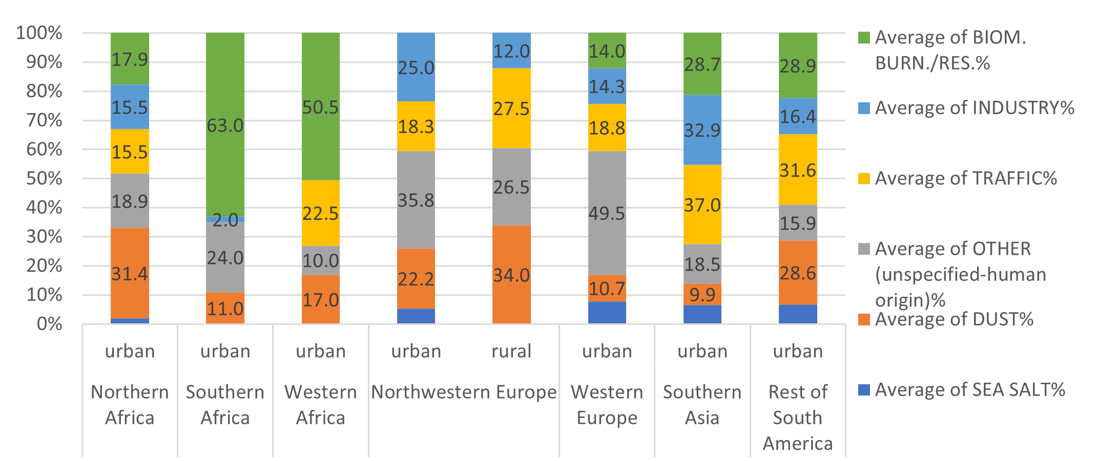
Source: WHO database on local source apportionment studies

CPAT can combine the information from source apportionment studies with the source apportionment result from applying the TM5-FASST coefficients. For each sector, we estimate an adjustment factor, \(\text{AF}_{s},\) to TM5-FASST coefficients, such that the external source contribution by sector will be met in the baseline year \(\text{to}\). The adjustment factor for each sector \(s\) is calculated as:

\[\text{AF}_{s} = \frac{\text{ShareFASST}_{s,to}}{\text{ShareExterna}l_{s}} \tag{6.13}\]

Where:

\(\text{AF}_{s}\): Adjustment factor for sector \(s\) (\(s\)= coal power plants, gas power plants, other power plants, ground level road, residential-construction-services, agriculture, other sectors).

\(\text{ShareFASS}T_{s}\): % Contribution to ambient PM_2.5 from sector \(s\), calculated using FASST coefficients

\(\text{ShareExterna}l_{s}\): % Contribution to ambient PM_2.5 from sector \(s\), according to user’s input or to WHO database.

The modeled ambient PM_2.5 under this option in CPAT is calculated as follows.

\[\text{Modeled~PM}{2.5}_{t} = \sum_{p}^{}{\sum_{s}^{}{AF_{s}*\text{FASST}_{p,s}*Emissions_{p,s,t}}} \tag{6.14}\]

In CPAT, we have uploaded the source apportionment information for the 46 countries included in the WHO database, as well as additional studies covering additional countries (see Table 6.9 for the country coverage of each study). The correspondence between the sectors in the WHO database and CPAT air pollution sectors is presented in Table 6.8.

Table 6.8: Matching from WHO database sectors and CPAT air pollution tab sectors

WHO database sectors	CPAT AP sectors
Industry	Coal Power Plants
Industry	Gas Power Plants
Industry	Other Power Plants
Traffic	Road transport
Industry / Domestic fuel burning	Residential, services and construction
Industry	Industries and other energy
Unspecified source of human origin	Food & forestry (includes agriculture)
Natural sources (dust and sea salt)	Unknown (not modeled, natural, outside borders)

Source: Own elaboration. The WHO sector “Unspecified source of human origin” includes secondary formation of PM_2.5 and it’s distributed among all CPAT sectors, including the “unknown” category in the proportions of each sector calculated using FASST coefficients.

CPAT allows the user to input other source apportionment distribution (manual input) and also includes a default distribution for most countries, based in the WHO database. The default source apportionment distribution is equal to the regional average, that can be used if the country is not covered in the WHO database. The information source used is indicated in the Air pollution module, under the section “Calibration options from the Dashboard/MSTInputs tab”.

Table 6.9 presents the country coverage of each of the studies preloaded in CPAT.

Table 6.9: Countries covered by source apportionment studies in CPAT

Study	Countries covered
World Health Organization (2015)	Argentina, Australia, Bangladesh, Belgium, Brazil, Canada, Chile, China, Costa Rica, Denmark, Egypt, Estonia, Finland, France, Germany, Ghana, Greece, India, Indonesia, Ireland, Italy, Japan, Korea, Kuwait, Macedonia, FYR, Malaysia, Mexico, Mongolia, Netherlands, New Zealand, Norway, Pakistan, Philippines, Poland, Portugal, Saudi Arabia, South Africa, Spain, Sri Lanka, Sweden, Switzerland, Thailand, Turkey, United Kingdom, United States, Vietnam
World Bank (2020)	Bosnia and Herzegovina
Almeida et al. (2020)	Greece, Kazakhstan, Hungary, Moldova, Croatia, Serbia, Albania, Bosnia and Herzegovina, Poland, Macedonia, FYR, Tajikistan
Lelieveld et al. (2015)	China, Tukey
World Bank (2019a)	Macedonia
Gaita et al. (2014)	Kenya (assumed same results for Rwanda)

6.5.4 Option 3: Elastic Net model and OLS model

CPAT also offers the option to apply the results of an elastic net regularization method to link emissions by sector to ambient concentrations of PM_2.5 and O₃ (Renna and Reis (2021)). The ambient concentrations predicted represent population weighted averages per country. At the moment CPAT offers the elastic net model option only for PM_2.5.

The results of the elastic net model are combined with an OLS model. The results of the OLS model are used only to distribute the contribution of modeled PM_2.5 among CPAT sectors, while the elastic net model is used to predict total ambient concentrations of PM_2.5.

The following table summarizes the data sources used to develop the elastic net and OLS models.

Variable	Data source
Emissions	CAMS Global Anthropogenic v4.2, 2000-2020, monthly, 0.1°
Concentrations	CAMS Global Reanalysis (EAC4) monthly averaged fields (Inness et al. (2019)), for 2003-2019, PM2.5 and Ozone
Population	2020 UN WPP-Adjusted Population Count, v4.11, from the NASA Socioeconomic Data and Applications Center (SEDAC) (CIESIN 2020).
Climate variables	Monthly data, 0.1 degrees resolution from TerraClimate. Variables used: precipitation, maximum temperature, minimum temperature, wind speed, vapor pressure deficit in kPa. Wind direction from ERA-5 Reanalysis Monthly Means

Source: Based on Renna and Reis (2021)

The model considers the emissions of BC, OC, NH3, SO2 and NMVOC. The sectoral aggregation of the models is the following:

• AGR (Agriculture)

  • Agricultural waste burning

  • Agriculture livestock

  • Agriculture soils

• ROA (Road transportation)

  • Road transportation

• INX (industry)

  • Industrial process

• POW (Energy Power generation)

  • Power generation

  • Fugitives

• SER (Buildings including residential, commercial and services)

  • Residential and other sectors

• OTR (Off-road transportation)

  • Off Road transportation

• OTH (Others, including the emissions not considered in the sectors above)

  • Solid waste and wastewater

  • Solvents

The data sources and methods are described in more detail in Renna and Reis (2021). In the next subsections we describe the implementation of the elastic net and OLS models in CPAT.

6.5.4.1 Elastic net model

As mentioned above, the elastic net model is used to predict total ambient PM_2.5 in CPAT. The functional form and the adaptations made to the original coefficients of the model is detailed in the following paragraphs.

Monthly concentrations of PM2.5

The linear regressions developed to predict monthly levels of PM_2.5 takes the form indicated in expression Equation 6.15 for each country.

\[P{M2.5}_{m} = \alpha + \sum_{s,p}^{}{\beta_{s,p}*E_{s,p,m}} + \gamma_{1}*PPT_{m} + \gamma_{2}*TMIN_{m} + \gamma_{3}*TMAX_{m} + \gamma_{4}*\text{VPD}_{m} + \gamma_{5}*\text{WS}_{m} + \gamma_{6}*\text{WD}_{m} + \sum_{s}^{}{{\delta_{s}*T}_{s,m} + \sum_{p}^{}{\lambda_{p}*T_{p,m}}} + \mu*T_{nox,m}*T_{NH3,m} + \nu*T_{SO2,m}*T_{NH3,m} + \xi*T_{SO2,m}*T_{NOx,m} + {\sum_{s}^{}{{\theta_{s}*T_{s,m}*WS}_{m}*WD_{m}} + \phi}_{m} + \varepsilon_{m} \tag{6.15}\]

Where:

\(m\) = Months of the year, from 1 to 12

\(s\ \in \{ agr,\ roa,\ pow,\ inx,\ otr,\ oth,\ ser\}\)

\(p\ \in \left\{ BC,\ OC,\ NH_{3},\ NO_{x},\ NMVOC,\ SO_{2} \right\}\)

\(P{M2.5}_{m}\) = Concentration of PM_2.5 in month \(m\), in \(\mu g/m^{3}\)

\({O3}_{m}\) = Concentration of \(O_{3}\) in month \(m\), in \(6mDMA8h\)⁸

\(E_{s,p,m}\) = Emissions of sector \(s\) and pollutant \(p\) in month \(m\), in \(Tg\)

\(\text{PP}T_{m}\) = Accumulated precipitation in mm, month \(m\)

\(\text{TMI}N_{m}\) = Minimum temperature in \(\deg{C}\) month \(m\)

\(\text{VP}D_{m}\) = Mean vapor pressure deficit in kPa, month \(m\)

\(WS_{m}\) = wind speed in \(\frac{m}{s}\), month \(m\)

\(WD_{m}\) = Wind direction in degrees, month \(m\)

\(T_{p,m}\) = composite index from the sum of total emissions of pollutant \(p\), in month \(m\)

\(T_{s,m}\) = composite index from the sum of total emissions of sector \(s\), in month \(m\)

\(\phi_{m}\) = Monthly fixed effects

\(\varepsilon\) = Error term

Annual concentrations of PM2.5

In CPAT, we work on an annual basis, while the elastic net model was developed to predict PM_2.5 in a monthly basis. Thus, we adapt the elastic net model results to predict annual concentration of PM_2.5, as explain below.

Each month of the year will have a weight according to its number of days, equal to \(\varphi_{m}\). For instance, for February, it’s weight in the annual average is \(\varphi_{2} = 28/365\).

The weighted average PM_2.5 will be calculated according to expression .

\[PM2.5 = \sum_{m}^{}{\varphi_{m}*PM{2.5}_{m}} \tag{6.16}\]

Which can be written as expression Equation 6.17.

\[PM2.5 = \alpha + \sum_{s,p}^{}{\beta_{s,p}*\overline{E_{s,p}}} + \gamma_{1}*\overline{\text{PPT}} + \gamma_{2}*\overline{\text{TMIN}} + \gamma_{3}*\overline{\text{TMAX}} + \gamma_{4}*\overline{\text{VPD}} + \gamma_{5}*\overline{\text{WS}} + \gamma_{6}*\overline{\text{WD}} + \sum_{s}^{}{{\delta_{s}*T}_{s}*\sum_{m}^{}{\varphi_{m}*w_{s,m}} + \sum_{p}^{}{\lambda_{p}*T_{p}}}*\sum_{m}^{}{\varphi_{m}*w_{p,m}} + \mu*T_{\text{NOx}}*T_{NH3}*\sum_{m}^{}{\varphi_{m}*w_{NOx,m}*w_{NH3,m}} + \nu*T_{SO2}*T_{NH3}*\sum_{m}^{}{\varphi_{m}*w_{SO2,m}*w_{NH3,m}} + \xi*T_{SO2}*T_{\text{NOx}}*\sum_{m}^{}{\varphi_{m}*w_{SO2,m}*w_{NOx,m}} + \sum_{s}^{}{\theta_{s}*T_{s}*\sum_{m}^{}{\varphi_{m}*w_{s,m}*WS_{m}*WD_{m}}} + \overline{\phi} + \varepsilon_{m} \tag{6.17}\]

Where:

\(\overline{E_{s,p}}\) = average (simple) monthly emissions of sector \(s\) and pollutant \(p\)

\(\overline{\text{PPT}}\) = average (weighted) monthly precipitations

\(\overline{\text{TMIN}}\) = average (weighted) \(TMIN\)

\(\overline{\text{TMAX}}\) = average (weighted) \(TMAX\)

\(\overline{\text{VPD}}\) = average (weighted) vapor pressure deficit

\(\overline{\text{WS}}\) = average (weighted) wins speed

\(\overline{\text{WD}}\) = average (weighted) wind direction

\(\overline{\phi}\) = average (weighted) monthly fixed effect

\(T_{p}\) = composite index from the sum of total emissions of pollutant p in all the months of the year$

\(w_{p,m}\) = share of emissions of pollutant \(p\) in month \(m\), \(T_{p,m}\), such that \(sum_{m = 1}^{12}{w_{p,m} = 1}\).

\(T_{s}\) = composite index from the sum of total emissions of sector \(s\) in all the months of the year

\(w_{s,m}\) = share of emissions of sector \(s\) in month \(m\), \(T_{s,m}\), such that \(sum_{m = 1}^{12}{w_{s,m} = 1}\).

Annual concentration of PM2.5 in CPAT

In CPAT, we group and consider constant all the weather variables, together with the intercept of the model and monthly fixed effects.

For each country, we define a weather constant equal to:

\[{Weather = \gamma}_{1}*\overline{\text{PPT}} + \gamma_{2}*\overline{\text{TMIN}} + \gamma_{3}*\overline{\text{TMAX}} + \gamma_{4}*\overline{\text{VPD}} + \gamma_{5}*\overline{\text{WS}} + \gamma_{6}*\overline{\text{WD}} \tag{6.18}\]

Where \(\overline{\text{VAR}} = \sum_{m}^{}{\varphi_{m}*\text{VAR}_{m}}\)

We define new constants, according to expressions Equation 6.19 to Equation 6.26.

\[\delta_{s}^{'} = \delta_{s}*\sum_{m}^{}{\varphi_{m}*w_{s,m}} \tag{6.19}\] \[\lambda_{p}^{'} = \lambda_{p}*\sum_{m}^{}{\varphi_{m}*w_{p,m}} \tag{6.20}\] \[\mu' = \mu*\sum_{m}^{}{\varphi_{m}*w_{NOx,m}*w_{NH3,m}} \tag{6.21}\] \[\nu' = \nu*\sum_{m}^{}{\varphi_{m}*w_{SO2,m}*w_{NH3,m}} \tag{6.22}\] \[\xi' = \xi*\sum_{m}^{}{\varphi_{m}*w_{SO2,m}*w_{NOx,m}} \tag{6.23}\] \[{{\theta^{'}}_{s} = \theta}_{s}*\sum_{m}^{}{\varphi_{m}*w_{s,m}*WS_{m}*WD_{m}} \tag{6.24}\] \[{\beta'}_{s,p} = \beta_{s,p}/12 \tag{6.25}\] \[{\beta''}_{s,p} = {(\beta'}_{s,p}{+ \lambda'}_{p}) \tag{6.26}\]

And we estimate annual PM_2.5 using expression Equation 6.27.

\[PM2.5 = \alpha + Weather + \overline{\phi} + \sum_{s,p}^{}{\beta_{s,p}*\overline{E_{s,p}}} + \sum_{s}^{}{{{\delta'}_{s}*T}_{s} + \sum_{p}^{}{{\lambda'}_{p}*T_{p}}} + \mu'*T_{\text{NOx}}*T_{NH3} + \nu'*T_{SO2}*T_{NH3} + \xi'*T_{SO2}*T_{\text{NOx}} + \sum_{s}^{}{{\theta'}_{s}*T_{s}} + \varepsilon_{m} \tag{6.27}\]

The contribution of each sector to PM_2.5 will be calculated according to expression Equation 6.28.

\[\text{PM}{2.5}_{s} = \sum_{p}^{}{{\beta'}_{s,p}*T_{p,s}} + {{\delta'}_{s}*T}_{s} + \sum_{p}^{}{{\lambda'}_{p}*T_{p,s}} + \mu'*T_{NOx,s}*T_{NH3,s} + \nu'*T_{SO2,s}*T_{NH3,s} + \xi'*T_{SO2,s}*T_{NOx,s} + {\theta'}_{s}*T_{s} \tag{6.28}\]

Grouping terms, we can write the contribution to PM_2.5 by sector as indicated in expression Equation 6.29.

\[\text{PM}{2.5}_{s} = \sum_{p}^{}{{(\beta'}_{s,p}{+ \lambda'}_{p})*T_{p,s}} + {({\delta^{'}}_{s} + {\theta^{'}}_{s})*T}_{s} + \mu'*T_{NOx,s}*T_{NH3,s} + \nu'*T_{SO2,s}*T_{NH3,s} + \xi'*T_{SO2,s}*T_{NOx,s} \tag{6.29}\]

Let’s call \({\beta''}_{s,p} = {(\beta'}_{s,p}{+ \lambda'}_{p})\) and \({\delta^{''}}_{s} = ({\delta^{'}}_{s} + {\theta^{'}}_{s})\) and write \(\text{PM}{2.5}_{s}\) as in expression Equation 6.30.

\[\text{PM}{2.5}_{s} = \sum_{p}^{}{{\beta''}_{s,p}*T_{p,s}} + {{\delta''}_{s}*T}_{s} + \mu'*T_{NOx,s}*T_{NH3,s} + \nu'*T_{SO2,s}*T_{NH3,s} + \xi'*T_{SO2,s}*T_{NOx,s} \tag{6.30}\]

Where:

\(T_{p,s}\) = composite index from the sum of total emissions of pollutant \(p\) in sector \(s\), including all the months of the year

The term \(\alpha + Weather + \overline{\phi} + \varepsilon_{m}\) is not sector specific and it is considered a constant in CPAT.

The term Equation 6.31 is also non-sector specific and is relating the interactions across emissions of the different sectors.

\[\mu'*(T_{\text{NOx}}*T_{NH3} - \sum_{s}^{}{T_{NOx,s}*T_{NH3,s}}) + \nu'*{(T}_{SO2}*T_{NH3} - \sum_{s}^{}{T_{SO2,s}*T_{NH3,s}}) + \xi'*(T_{SO2}*T_{\text{NOx}} - \sum_{s}^{}{T_{SO2,s}*T_{NOx,s}}) \tag{6.31}\]

6.5.4.2 OLS model

As mentioned before, in CPAT we apply the results of an OLS model to quantify the percent contribution of each sector to ambient PM_2.5, while we use the elastic net model to predict total concentrations.

The OLS model has the functional form in expression Equation 6.32.

\[P{M2.5}_{m} = \alpha + \sum_{s}^{}{\delta_{s}*\widehat{T_{s,m}}} + \gamma_{1}*PPT_{m} + \gamma_{2}*TMIN_{m} + \gamma_{3}*TMAX_{m} + \gamma_{4}*\text{VPD}_{m} + \gamma_{5}*\text{WS}_{m} + \gamma_{6}*\text{WD}_{m} + \varepsilon_{m} \tag{6.32}\]

Where \(\widehat{T_{s,m}}\) is a composite index of total normalized emissions in month \(m\) and sector \(s\). The procedure to normalize emissions is explained below.

Normalization of emissions for OLS model

For each country, let’s call normalized emissions by sector and pollutant and month, \(\widehat{E_{s,p,m}}\), that is calculated using expression Equation 6.33.

\[\widehat{E_{s,p,m}} = \frac{E_{s,p,m} - \text{Min}_{s,p}}{\text{Max}_{s,p} - \text{Min}_{s,p}} \tag{6.33}\]

Where:

\(E_{s,p,m}\): emissions in month \(m\) per pollutant \(p\) and sector \(s\)

\(\text{Min}_{s,p}\): Min emission across months for pollutant \(p\) and sector \(s\)

\(\text{Max}_{s,p}\): Max emission across months for pollutant \(p\) and sector \(s\)

Then, the index \(\widehat{T_{s,m}}\) is calculated using expression Equation 6.34.

\[\widehat{T_{s,m}} = \sum_{p}^{}\widehat{E_{s,p,m}} \tag{6.34}\]

In CPAT, we do not calculate monthly emissions, but annual emissions, thus, the normalization of emissions and the index of total normalized emissions by sector considers annual emissions by sector and pollutant.

6.5.5 Option 4: Intake fractions

Another option in CPAT to relate emissions to ambient concentration of PM_2.5 is using intake fractions. Intake fractions were defined in Bennett et al. (2002) as the integrated incremental intake of a pollutant, summed over all exposed individuals, and occurring over a given exposure time, released from a specified source or source class, per unit of pollutant emitted. Intake fractions measure the change in population-weighted ambient concentrations of a pollutant (PM_2.5 in this case) per unit of pollutant emitted Cropper et al. (2012). Zhou et al. (2006) defined intake fractions as the fraction of material or its precursors released from a source that is eventually inhaled or ingested by a population. Intake fractions are defined by Equation 6.35.

\[iF = \frac{\sum_{i = 1}^{N}{P_{i}*\mathrm{\Delta}C_{i}*BR}}{Q} \tag{6.35}\]

Where:

\(\text{iF}\): Intake Fraction, inhaled grams of PM_2.5 per ton (ppm) of emissions

\(P_{i}\): population residing in a region located at a distance \(i\) from the emission source

\(\text{ΔC}_{i}\): change in ambient concentration of PM_2.5 g/m³

\(\text{BR}\): Average breathing rate in cubic meters per day m³/day

\(Q\): Emissions rate tonne/day

From Equation 6.35, rearranging the terms, we can express changes in concentration weighted average as shown in Equation 6.36.

\[\sum_{i = 1}^{N}{P_{i}*\mathrm{\Delta}C_{i}} = \frac{iF*Q}{\text{BR}} \tag{6.36}\]

Intake fractions are influenced by the emissions height, as illustrated in Figure 6.10. Ground level emissions are usually inhaled in a major proportion, compared with emissions from a high stack.

Figure 6.10: Illustration of Intake fraction variation according to emissions height

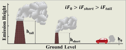
Source: Parvez, Lamancusa, and Wagstrom (2017)

At the same time, intake fractions depend on the population density at different distances from the emission source. As illustrated in Figure 6.11, higher population concentrations will increase the intake fraction value, since more people is inhaling pollution.

Figure 6.11: Illustration of intake fractions variation according to distance from the source and population concentration.

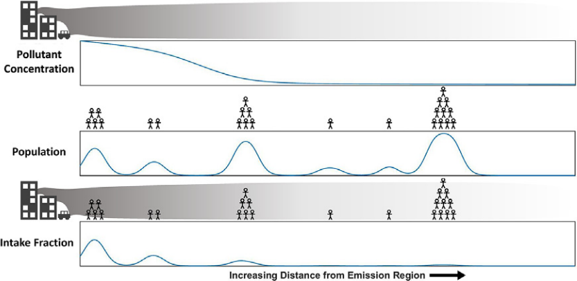
Source: Lamancusa, Parvez, and Wagstrom (2017)

6.5.5.1 Intake fractions for ground level, low and high stack emission sources

In CPAT, for sources different than power plants, we use the results from Apte et al. (2012). The study estimates intake fractions for more than 3,600 cities, for ground level sources and for direct emissions of PM_2.5.

In the case of secondary pollutants, we will scale up the ground-level secondary intake fractions from Humbert et al. (2011), presented in Table 6.10, using the ratio between primary PM_2.5 intake fractions from Apte et al. (2012) and Humbert et al. (2011), as indicated in Equation 6.37.

\[\text{iF}_{\text{secondary\ pollutant}} = \frac{\text{iF}_{PM2.5,\ Apte}}{\text{iF}_{PM2.5,\ Humbert}}*\text{iF}_{\text{secondary\ Humbert}}\ \tag{6.37}\]

Table 6.10: Intake fractions (ppm) for ground level PM_2.5

Pollutants		Urban	Rural	Remote
Primary PM2.5	Ground-level PM2.5	44	3.8	0.1
	high-stack	11	1.6	0.1
	low-stack	15	2.0	0.1
Secondary PM2.5	SO2	0.99	0.79	0.05
	NOx	0.2	0.17	0.01
	NH3	1.7	1.7	0.1

Source: Humbert et al. (2011)

For non-ground level sources, in which emissions take place trough high or low stacks, the \(iF\) is estimated according to Equation 6.38.

\[\text{iF}_{high/low} = \text{iF}_{PM2.5,\ Fantke}*\frac{\text{iF}_{PM2.5,\ \ Humbert,\ high/low}}{\text{iF}_{PM2.5,\ Humbert,\ \ groundlevel}} \tag{6.38}\]

6.5.5.2 Intake fractions from power plants

Power plants emissions are released from tall smokestacks and consequently are likely to be transported long distances. In order to include the geographically extended effect of power plants emissions into the analysis, we will use intake fractions that were developed specifically for this sector, following Zhou et al. (2006).

Zhou et al. (2006) estimates intake fractions for 29 power plants in China and proposes a methodology to calculate intake fractions in other regions of the world using population and precipitation data. The authors extrapolated the intake fraction results to other sites using regression analysis (see Table 6.11). This methodology (Zhou et al. (2006)) was applied by on the spreadsheet model developed by Parry et al. (2014) and subsequent IMF iterations.

CPAT intake fractions use updated data regarding power plant’s location and population distribution around them, together with differentiating exposed population inside country borders and outside countries. The methodology is illustrated in Figure 6.12.

Figure 6.12: Methodology for estimating intake fractions for power plants

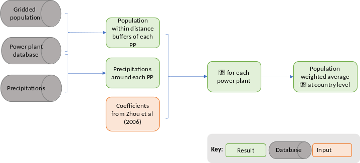
Source: Own elaboration

The following table provides a comparison between the approach implemented by Parry et al. (2014) and CPAT.

	Parry 2014	CPAT
Methodology	Coefficients from Zhou et al. (2006) (Table 4)	Coefficients from Zhou et al. (2006) (Table 6)
Power plants data	CARMA 2009 data. 110 countries 2,400 coal plants 2,000 natural gas plants	Global Power Plant Database9 (Global Energy Observatory, Google, KTH Royal Institute of Technology in Stockholm, Enipedia, World Resources Institute (2018)). Updated in 2019 164 countries 2,390 coal plants 3,922 gas power plants 2,290 oil power plants
Gridded population	LandScan- 2010 Population	Earth Data10, 2020 pop (Center for International Earth Science Information Network (CIESIN) Columbia University 2018b)
Exposed population	Population within 2000 km (above 25). No distinction between inside and outside the country	Population within 2000 km (distributed in age ranges). Distinction between inside and outside (relevant for country analysis).
Precipitations	-	Precipitations
Breathing rate	20 m3/day (from Zhou et al. (2006))	20 m3/day
Weight for averages at country level	Coal used (based on CO2 emissions)	Power generation (average years available or estimated generation). If no value for generation, then we assigned a simple average.

As indicated in the previous table, CPAT will use the Global Power Plant Database (Global Energy Observatory, Google, KTH Royal Institute of Technology in Stockholm, Enipedia, World Resources Institute (2018)), which includes approximately 28,700 geolocated power plants in 164 countries, accounting for 80% of global installed capacity (Byers et al. (2018)). The database contains 2,390 coal plants, 3,922 gas power plants and 2,290 oil power plants.

The team decided to use this database, since CARMA database has not been updated since 2012 (Byers et al. (2018)). Figure 6.13 shows, as an example, the location of the coal power plants included in the database.

Figure 6.13: Location of Coal Power Plants

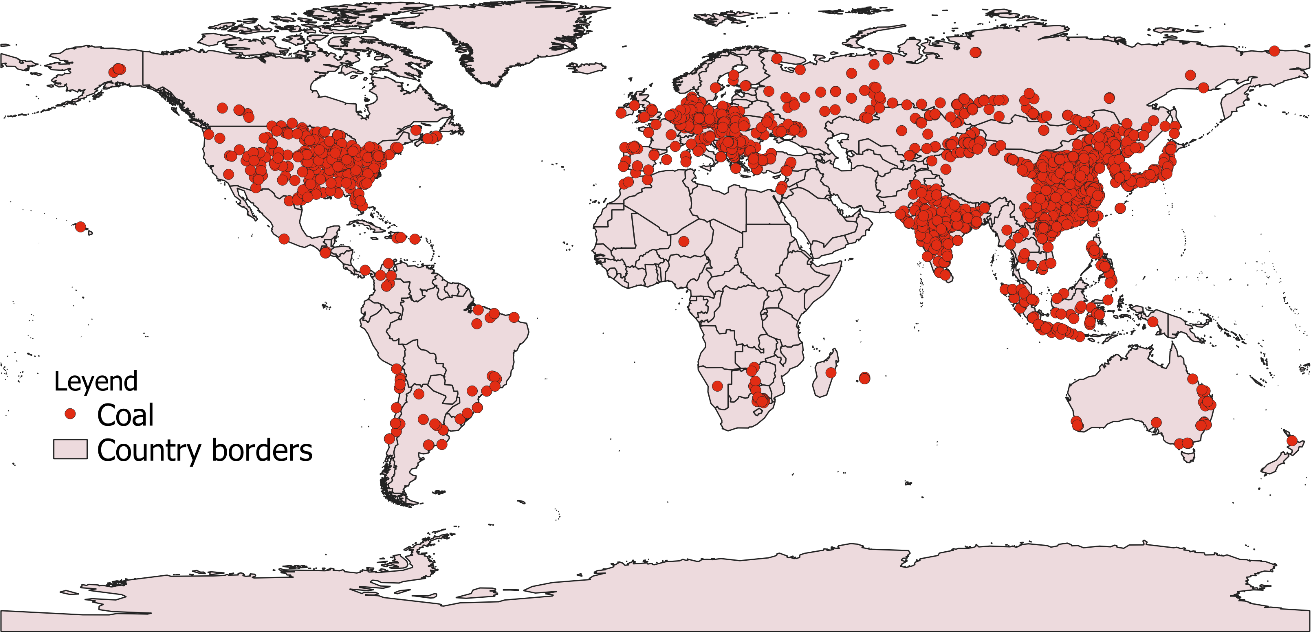
Source: Based on Global Energy Observatory, Google, KTH Royal Institute of Technology in Stockholm, Enipedia, World Resources Institute (2018) ¹¹

Zhou et al. (2006) requires estimating population around different distances of each power plant. To estimate population inside different distance buffers, gridded population data was obtained from the Center for International Earth Science Information Network (CIESIN), from Columbia university. The population-count raster file used consists of estimates of human population (number of persons per pixel), consistent with national censuses and population registers, for the years 2000, 2005, 2010, 2015, and 2020 (CPAT analysis is based on 2020). The data set consists of global raster files at 30 arc-second horizontal resolution (approximately 1 km at the equator). The 30 arc-second¹² data were aggregated to 2.5 arc-minute, 15 arc-minute, 30 arc-minute and 1 degree resolutions (Center for International Earth Science Information Network - CIESIN - Columbia University (2018)). The team decided to use this dataset, instead of Landscan 2017, since the former is available free of charge, and both sources provide equivalent quality and resolution.

The methodology in Zhou et al. (2006) allows the inclusion of the variable precipitations. Precipitations data¹³ was obtained from The Millennium Ecosystem Assessment (MA) Climate and Land Cover, v1 (1901 – 2000)¹⁴ (Reid and Raudsepp-Hearne (2005)). This dataset contains raster grids for monthly average precipitations.

For each power plant, we built a distance buffer of 40 kilometers and we compute the average precipitation inside that buffer. That variable is then used to predict intake fractions for each power plant, according to in Zhou et al. (2006).

The regression coefficients from Zhou et al. (2006), presented in Table 6.11, will be used to estimate an intake fraction for each power plant in each country.

Table 6.11: Coefficients for intake fractions from Zhou et al. (2006), Table 6

Pollutant \(\mathbf{j}\)	R2	\(\mathbf{\beta}_{\mathbf{1}}\) - Population within 100 km	\(\mathbf{\beta}_{\mathbf{2}}\) - Population between 100 and 500 km	\(\mathbf{\beta}_{\mathbf{3}}\) - Population between 500 and 1000 km	\(\mathbf{\beta}_{\mathbf{4}}\) - Population beyond 1000 km	\(\mathbf{\beta}_{\mathbf{5}}\) - Precipitation
SO2	0.96	9.90E-08	**	1.30E-08	**	3.00E-09		1.80E-09	**	-6.30E-10
PM1	0.96	1.50E-07	*	2.30E-08	**	1.10E-08	**	3.90E-09	**	-1.70E-09	**
PM3	0.92	1.40E-07	*	1.70E-08	**	6.40E-09		3.00E-09	**	-2.40E-09	**
PM7	0.91	9.90E-08	**	8.90E-09	*	3.10E-09		1.50E-09	*	-1.20E-09	*
PM13	0.89	6.70E-08	**	4.30E-09		9.40E-10		7.30E-10		-4.60E-10
SO4	0.95	2.40E-08		7.90E-09	*	6.90E-09	**	2.60E-09	**	-1.20E-09	**
NO3	0.93	4.30E-08		1.30E-08	**	3.50E-09		2.50E-09	**	-1.90E-09	**

Source: Zhou et al. (2006).

Notes: Estimate significant at 0.05 level. Estimate significant at 0.10 level. Population variables in millions; precipitation in mm/yr

The intake fraction for each power plant is calculated according to Equation 6.39, using the coefficients from Table 6.11.

\[{iF}_{p,\ j,\ l} = \sum_{i = 1}^{4}{\beta_{i,j}*{P\text{op}}_{i,\ l} + \beta_{5,\ j}*{P\text{recipitation}}_{p}} \tag{6.39}\]

Where:

\({iF}_{p,\ j,\ c}\): Intake fraction for power plant \(p\), pollutant \(j\), location \(l\)

\({P\text{op}}_{i,\ l}\): Population at distance \(i\), location \(l\)

\({P\text{recipitation}}_{p}\): Precipitations around plant \(p\)

\(\beta_{i,j}\): Regression coefficients for pollutant \(j\), location \(l\)

\[i = \left\{ \begin{matrix} \ \ \ \ 1,\ \ Population\ within\ 100\ km\ \ \ \ \ \ \ \ \ \ \ \ \ \ \ \ \ \ \ \ \ \ \ \ \\ 2,\ \ Population\ between\ 100\ and\ 500\ km\ \ \ \\ 3,\ \ Population\ between\ 500\ and\ 1000\ km \\ 4,\ \ Population\ within\ 1000\ and\ 2000\ km\ \\ \end{matrix} \right.\ \]

\(j\)= SO₂, PM₁, PM₃, PM₇, PM₁₃, SO₄, NO₃

\(l\) = inside country, outside country

Then, country level averages will be computed as the weighted average of the \(\text{iF}\) of each plant located inside the country, using as the weight the power generation¹⁵ of each power plant.

Finally, we calculate the changes in PM_2.5 concentrations rearranging the terms in Equation 6.35, assuming that the entire population is exposed to the weighted average concentration. We also adjust the units to obtain changes in concentration in µg/m³. \(\text{CM}\) corresponds to the implied “concentration matrix” that relates changes in concentration derived from 1 ton of emissions per year.

\[CM = \frac{\Delta C\lbrack\frac{\text{μg}}{m3}\rbrack}{1\ \lbrack tonne/year\rbrack} = \frac{iF\ (ppm)}{\text{BR}\left( \frac{m3}{d} \right)*365\left( \frac{d}{\text{year}} \right)*Pop\ (capita)}*10^6 \tag{6.40}\]

Where \(\text{ΔC}\) is the change in ambient concentration of PM_2.5, \(\text{iF}\) is a national level average intake fraction, \(\text{BR}\) is an average breathing rate and \(\text{Pop}\) is the country’s population.

6.5.6 Option 5: Machine learning

The user can also choose to use the results of a machine learning approach, developed for CPAT Renna and Reis (2021). The results of the model have been approximated using a discrete function, that relates emissions perturbations to total ambient concentrations of PM_2.5 and O3.

\(P_{s,p,t}\) is the perturbation compared to emissions in the baseline year, \(t_{0}\), in percentage. We use 2019 as the baseline year and all the perturbations are compared to that year, as presented in Equation 6.41.

\[P_{s,p,t} = \ \left( \frac{\text{Emission}s_{s,p,t}}{\text{Emissions}_{s,p,t0}} - 1 \right)*100 \tag{6.41}\]

Total ambient concentration is a function of \(P_{s,p,t}\), composed of a set of linear relationships, according to the level of the perturbation, as presented in Equation 6.42.

\[ C\ (P_{s,p,t}) = \left\{\begin{matrix} \\\\ \text{if } P_{s,p,t} < -100, \ a_{-100} \\ \text{if } -100 \le P_{s,p,t} < -80,\ \ \ a_{- 100} + b_{- 100}*(P_{s,p,t} - ( - 100)) \\ \text{if } - 80 \leq P_{s,p,t} < - 60,\ \ \ a_{- 80} + b_{- 80}*(P_{s,p,t} - ( - 80)) \\ \text{if } - 60 \leq P_{s,p,t} < - 40,\ \ \ a_{- 60} + b_{- 60}*(P_{s,p,t} - ( - 60)) \\ \text{if } - 40 \leq P_{s,p,t} < - 20,\ \ \ a_{- 40} + b_{- 40}*(P_{s,p,t} - \left( - 40 \right)) \\ \text{if } - 20 \leq P_{s,p,t} < 0,\ \ \ a_{- 20} + b_{- 20}*(P_{s,p,t} - \left( - 20 \right)) \\ \text{if }\ 0 \leq P_{s,p,t} < 20,\ \ \ a_{0} + b_{0}*(P_{s,p,t} - 0) \\ \text{if }\ 20 \leq P_{s,p,t} < 40,\ \ \ a_{20} + b_{20}*(P_{s,p,t} - 20) \\ \text{if }\ 40 \leq P_{s,p,t} < 60,\ \ \ a_{40} + b_{40}*(P_{s,p,t} - 40) \\ \text{if }\ 60 \leq P_{s,p,t} < 80,\ \ \ a_{60} + b_{60}*(P_{s,p,t} - 60) \\ \text{if }\ 80 \leq P_{s,p,t} < 100,\ \ \ a_{80} + b_{80}*(P_{s,p,t} - 80) \\ \text{if }P_{s,p,t} > 100,\ \ \ a_{100} + b_{100}*(P_{s,p,t} - 100) \\ \end{matrix} \right. \tag{6.42}\]

For the baseline year \(t_0\), the contribution of sector \(s\) and pollutant \(p\) to ambient PM_2.5 is presented in Equation 6.43. The mentioned contribution is equivalent to the change in ambient PM_2.5 when the emissions are reduced to zero (a -100% perturbation).

\[C_{s,p,t_0} = {- C}_{s,p,t}(P_{s,p,t} = - 100) \tag{6.43}\]

Then, the contribution in each year \(t\) of sector \(s\) and pollutant \(p\) to ambient PM_2.5 is presented in Equation 6.44.

\[C_{s,p,t} = C_{s,p,t}\left( P_{s,p,t} \right) - BaselineConcentration + C_{s,p,t_0} \tag{6.44}\]

The change in contribution to ambient PM_2.5 or Ozone is calculated by subtracting the contribution in the baseline and the contribution under the carbon policy scenario.

6.5.7 Option 6: Average between two methods

In addition to the options to relate emissions and concentrations described above, the user can select the average among two of the methods described: intake fractions (Section 6.5.5) and source-apportionment information combined with TM5-FASST method (Section 6.5.3). We added this option since every method used is subject to uncertainty and using more than one estimate will provide results in the middle range of different model estimates.

6.5.8 Modeled and total ambient pollution

In CPAT, we estimate emissions from the sectors and fuels presented in Table 6.1 according to the methodology described in Section 6.4. Then, using one of the six options described in Section 6.5, we determine the “modeled” ambient PM_2.5 (or O3). The modeled concentration accounts only for fuel burning activities, but not for all ambient pollution.

Other sources of pollution (not fuel burning) include resuspended dust, sea salt, forest fires, or other transboundary sources that contribute to observed PM_2.5. We assume that the sources not modeled in CPAT contribute a \(C_{0}\) level to ambient pollution. We calculate the value \(C_{0}\) for a baseline year, using Equation 6.45, and we assume it to remain constant across time.

\[\text{Observed}C_{t_0} = Modeled\ C_{t_0} + C_{0} \tag{6.45}\]

Total ambient concentration each year \(t\) is modeled in CPAT using expression Equation 6.46.

\[\text{Ambient}C_{t} = Modeled\ C_{t} + C_{0} \tag{6.46}\]

Figure 6.14 presents graphically the methodology applied: a constant \(C_{0}\) and a modeled concentration that varies in time.

Figure 6.14: Illustrative example of the projection in time of ambient PM_2.5 in CPAT

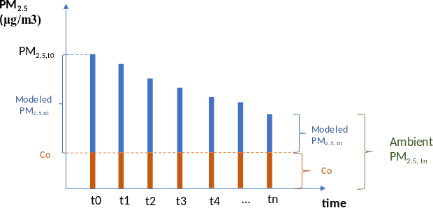
Source: Own elaboration

6.6 Methods to calculate the health burden of air pollution

This chapter describes the methodologies and data sources used to quantify the health impacts attributed to air pollution in CPAT. The health metrics described in this section, such as mortality, are the main result from the air pollution tab.

Figure 6.15: Health effects, CPAT methodology overview

Source: Own elaboration

The health burden of air pollution is quantified using the methodology illustrated in Figure 6.16. The health outcomes included in CPAT are premature mortality and disability-adjusted life years (DALYs), explained in the following sections.

Figure 6.16: Methodology for estimating the health burden of pollution

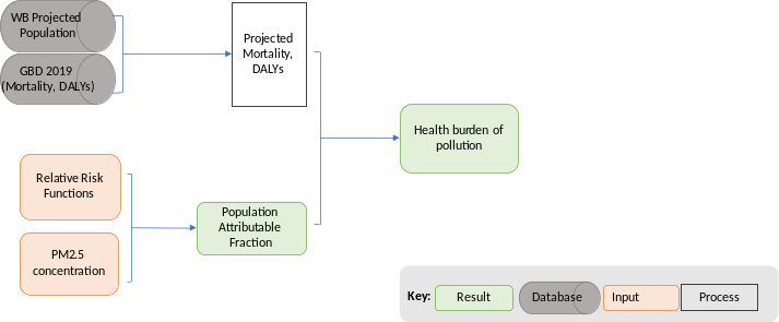
Source: Own elaboration

6.6.1 Data sources to estimate health impacts

Input	Source
Relative Risk estimates (by cause, age and exposure level)	Global Burden of Disease Health Financing Collaborator Network (2020)
Population projections by age group and country	WB Population Estimates and Projections16. The database includes population projections by country, sex and age range by country up to 2050. It also includes the share or urban and rural populations.
Urban population fraction by country	World Bank Group
Mortality and DALYs	Global Burden of Disease Health Financing Collaborator Network (2020) Mortality and DALYs for: Ischemic heart disease Chronic obstructive pulmonary disease Lower respiratory infections Stroke Tracheal, bronchus, and lung cancer Diabetes mellitus type II Neonatal diseases: Sudden infant death syndrome, Diarrheal diseases, Lower respiratory infections, Upper respiratory infections, Otitis media, Meningitis, Neonatal disorders, Encephalitis
Exposure to ambient PM2.5	WHO Country average exposure (World Health Organization (2018))17 and Global Burden of Disease Health Financing Collaborator Network (2020) ambient concentrations.
Exposure to indoors PM2.5	Data from the Global Burden of Disease Health Financing Collaborator Network (2020) study, provided by Michael Brauer
Exposure to ozone pollution	Data from the Global Burden of Disease Health Financing Collaborator Network (2020) study, provided by Michael Brauer

6.6.2 Definitions of key technical terms

Relative Risk (RR) is a measure of the change in risk of an adverse health effect associated with an increase in air pollution levels. RR indicates the likelihood of developing the disease of effect in the exposed group, relative to those who are not exposed.

\[\text{RR} = \frac{y_{0}}{y_{c}} \tag{6.47}\]

Where:

\(y_{0}\): the risk (or probability) that people with baseline pollutant exposure will be adversely affected

\(y_{c}\): the risk (or probability) that people with control pollutant exposure will be negatively affected.

For example, a RR for all-cause mortality equal to 1.03 per 10 µg/m3 increase in annual PM_2.5 means that a 10 µg/m3 increase in PM_2.5 is associated with a 3% increase in deaths from all causes.

Hazard represents an instantaneous event rate or the probability that an individual would experience an event at a given point in time.

Hazard Ratio is defined as the baseline hazard (\(H_{0}\)) divided by hazard in the control group (\(H_{c}\)).

\[\text{HR} = \frac{H_{0}}{H_{c}}\]

Hazard ratio is often interpreted as relative risk, but they are not technically the same. The main difference is that relative risk does not consider the timing of the event but only the occurrence of the event by the end of the observation period. The hazard ratio considers both.

Incidence corresponds to the number of new cases of a given disease during a given period in a specified population. It also is used for the rate at which new events occur in a defined population. It is differentiated from prevalence, which refers to all cases, new or old, in the population at a given time¹⁸.

\[\text{Incidence}\ \text{proportion} = \ \frac{\text{number}\ \text{of}\ \text{new}\ \text{cases}\ \text{in}\ \text{period}}{\text{population}\ \text{at the start of the}\ \text{period}}*10^5\]

Prevalence is the total number of cases of a given disease in a specified population at a designated time. It is differentiated from incidence, which refers to the number of new cases in the population at a given time¹⁹.

\[\text{Period}\ \text{Prevalence} = \ \frac{\text{number}\ \text{of}\ \text{prevalent}\ \text{cases}\ \text{in}\ \text{period}}{\text{number}\ \text{of}\ \text{individuals}\ \text{in}\ \text{period}}*10^5\]

The population attributable fraction (PAF) is the reduction in incidence that would be observed if the population were entirely unexposed, compared with its current exposure pattern. In other words, PAF is the portion of the incidence that could be reduced if causative exposure were eliminated

6.6.3 The health burden of pollution

The burden of disease associated with air pollution estimates the reduction in specific causes of death that would occur if the exposure were reduced to an alternative level (in general, the theoretical minimum risk level is used). The methodology combines information regarding population exposure to ambient air pollution and an exposure-response relationship.

Figure 6.17: Method for burden of disease estimation

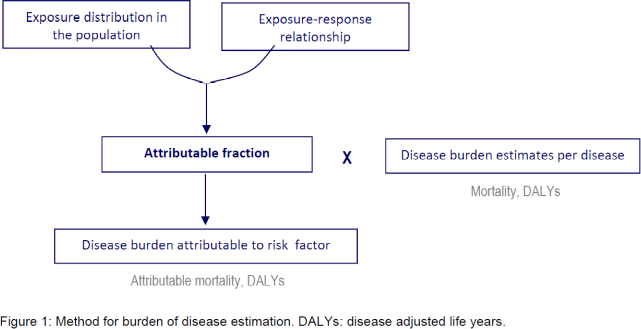
Source: World Health Organization and others (2018)

In CPAT, we implemented a method to assess jointly indoors and outdoors pollution as described in Section 6.6.4.1. CPAT also calculates the impacts of ozone pollution, as described in Section 6.6.4.3.

6.6.3.1 Joint ambient and household air pollution (Global Burden of Disease Health Financing Collaborator Network (2020))

In CPAT, we quantify the effects of air pollution following the methodology of the Global Burden of disease study for 2019 (Global Burden of Disease Health Financing Collaborator Network (2020)). The methodology uses and Integrated Exposure Response (IER) approach, basing its estimates in studies for ambient pollution, second-hand smoking and household pollution. This methodology represents and upgrade from the previous version of the study and the main differences with the previous methodology are the following:

• Global Burden of Disease Health Financing Collaborator Network (2020) no longer uses active smoking data in the risk curves. This removes an important source of uncertainty

• New studies in China and other high-exposure settings are now used²⁰

• No fixed functional form. Splines generated using MR-BRT (meta-regression boosted regression trees)

The methodology implemented in CPAT assess jointly the effects of ambient and household pollution. This feature is important because it allows the quantification of a possible increase in the use of solid fuels for cooking (leakage effects) and because household pollution is a major health problem in many countries of the world.

The relative risks used in CPAT from Global Burden of Disease Health Financing Collaborator Network (2020) are presented in Figure 6.18. In the case of ischemic heart disease and stroke, the RR presented is an average across all the age groups, which are defined in buckets of 5 years²¹. In CPAT, we work with the following age groups: neonates, post neonates, under 15, 15 to 64 and 65 years and above. We use the average relative risk withing each group.

Figure 6.18: RR from the Integrated exposure response function, Global Burden of Disease Health Financing Collaborator Network (2020)

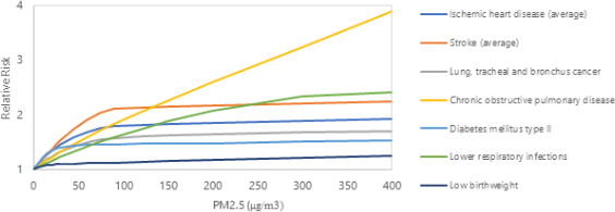
Notice that the relative risk takes as a reference the minimum risk level for PM_2.5, TMREL, defined as uniform distribution between 2.4 and 5.9 µg/m³. In CPAT, we use as the TMREL the average between 2.4 and 5.9, equal to 4.15 µg/m³ of PM_2.5. When pollution is below that level, we would obtain cero health effects attributed to pollution.

The diseases and age groups covered by the methodology in CPAT are presented in Table 6.12.

Table 6.12: Integrated Exposure Response function diseases from GBD 2019 implemented in CPAT

Cause	Age Group	RR
Chronic obstructive pulmonary disease	All ages	Constant across age groups
Diabetes mellitus type 2	All ages
Lower respiratory infections	All ages
Tracheal, bronchus, and lung cancer	All ages
Ischemic heart disease	Above 25	Changes with age
Stroke	Above 25
Low birthweight diseases22,23, excluding lower respiratory infections	Neonatal (under 28 days)	Constant

Source: Own elaboration. Note: GBD2019 also quantifies preterm birth²⁴ effects attributed to pollution. We do not quantify this in CPAT, to avoid double counting of effects, when aggregating the total impacts of pollution.

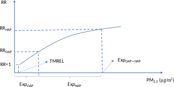
The joint methodology requires the fraction of the population that it is exposed to solid fuels for cooking, \(p_{\text{HAP}}\), and the level of exposure to household air pollution (HAP), as the additional exposure over and above ambient exposure to PM_2.5 (OAP).

For the proportion of the population not exposed to HAP, the relative risk is presented in Equation 6.48.

\[\text{RR}_{\text{OAP}} = MRBRT(z = \text{Exp}_{\text{OAP}})/MRBRT(z = TMREL) \tag{6.48}\]

For the proportion of the population exposed to HAP, the relative risk is given by Equation 6.49.

\[\text{RR}_{\text{HAP}} = MRBRT(z = \text{Exp}_{\text{OAP}} + \text{Exp}_{\text{HAP}})/\ MRBRT(z = TMREL) \tag{6.49}\]

The population level relative risk \(RR_{\text{PM}}\) and population attributable fraction, \(\text{PA}F_{\text{PM}}\), are calculated according to Equation 6.50 and Equation 6.51.

\[RR_{\text{PM}} = RR_{\text{OAP}}*\left( 1 - p_{\text{HAP}} \right) + RR_{\text{HAP}}*p_{\text{HAP}} \tag{6.50}\]

\[{PAF}_{\text{PM}} = 1 - 1/RR_{\text{PM}} \tag{6.51}\]

Finally, PAFs are split based on the exposure to OAP and HAP, as presented in Equation 6.52 and Equation 6.53.

\[\text{PA}F_{\text{OAP}} = \frac{\text{Exp}_{\text{OAP}}}{\text{Exp}_{\text{OAP}} + p_{\text{HAP}}*\text{Exp}_{\text{HAP}}}*\text{PAF}_{\text{PM}} \tag{6.52}\]

\[\text{PA}F_{\text{HAP}} = \frac{{p_{\text{HAP}}*Exp}_{\text{HAP}}}{\text{Exp}_{\text{OAP}} + {p_{\text{HAP}}*Exp}_{\text{HAP}}}*\text{PAF}_{\text{PM}} \tag{6.53}\]

Notice that under this strategy \(\text{PAF}_{\text{PM}} = \text{PAF}_{\text{HAP}} + \text{PAF}_{\text{OAP}}\).

Where:

\(\text{Exp}_{\text{OAP}}\): Ambient PM_2.5 exposure level

\(\text{Exp}_{\text{HAP}}\): Excess exposure to PM_2.5 for those who use solid fuel for cooking.

\(p_{\text{HAP}}\): proportion of the population using solid fuel for cooking

\(\text{RR}_{\text{OAP}}\): Relative risk for the proportion of the population not exposed to HAP

\(\text{RR}_{\text{HAP}}\): Relative risk for the proportion of the population exposed to HAP

\(RR_{\text{PM}}\): Population level relative risk

\(\text{PA}F_{\text{PM}}\): Population level PAF

Figure 6.19 presents a diagram of the exposure to PM_2.5, \(\text{Exp}_{\text{OAP}}\) and \(\text{Exp}_{\text{HAP}}\), and their associated relative risks levels.

Figure 6.19: Diagram for relative risk due to HAP and OAP exposure

Source: Own elaboration

The Attributable burden (\(\text{AB}\)) corresponds to the number of cases attributed to the exposure in the population. The AB is calculated by multiplying PAF by the baseline number of health outcomes, for each outcome, sex and age group.

\(AB = PAF*Health\ Outcome\)

The strategy to quantify health effects in CPAT is presented in Section 6.10.3.

6.6.3.2 Health outcomes in CPAT

In CPAT, we quantify the health effects of pollution as mortality, years of life lost, years lived with disability and disability-adjusted life years (DALYs).

DALY is a summary measure which combines time lost through premature death and time lived in states of less-than-optimal health or “disability”. Figure 6.20 presents an infographic about the DALY metric.

Figure 6.20: DALY or disability-adjusted life year infographic

Source: Wikimedia Commons contributors (2020)

DALY, for a specific cause \(c\), sex \(s\), age \(a\) and year \(t\) is defined as indicated in Equation 6.54.

\[\text{DALY}_{c,s,a,t} = \text{YLL}_{c,s,\ a,t} + \text{YLD}_{c,s,a,t} \tag{6.54}\]

The years of life lost (YLL) are calculated in Equation 6.55 as the number of deaths multiplied by a loss function specifying the years lost for deaths as a function of the age at which death occurs.

\[\text{YLL}_{c,s,\ a,t} = {\text{Number}\ \text{of}\ \text{deaths}}_{c,s,a,t}*L_{s,a} \tag{6.55}\]

Where \(L_{s,a}\) is a standard loss function specifying years of life lost for a death at age \(a\) for sex \(s\).

The years lived with disease (YLD) are measured by the multiplication of the prevalence of the condition²⁵ and a weight factor that reflects the severity of the condition on a scale from 0 (perfect health) to 1 (death) as expressed in Equation 6.56.

\[\text{YLD}_{c,s,a,t} = P_{c,s,a,t}*\text{DW}_{c,s,a} \tag{6.56}\]

Where,

\(P_{c,s,a,t}\): Prevalent sequelae for cause \(c\), sex \(s\), age \(a\) and year \(t\)

\(\text{DW}_{c,s,a}\): Disability weight for sequelae for cause \(c\), sex \(s\) and age \(a\)

CPAT uses incidence at a country level for DALYs, YLL and YLD from Global Burden of Disease Health Financing Collaborator Network (2020).

6.6.3.3 Ozone air pollution

For ozone health effects, CPAT follows the methodology applied in Global Burden of Disease Health Financing Collaborator Network (2020), which is based on Turner et al. (2016). The health impacts are quantified for chronic obstructive pulmonary disease, with a RR of 1.06 (1.02, 1.10) per 10 ppb of ozone, in the seasonal (six-month period with the highest mean) 8-h daily maximum concentration metric (6mDMA8h). The TMREL for ozone is defined as ~ U (29.1, 35.7).

The relative risk is represented by expression Equation 6.57 and PAF is calculated using expression Equation 6.58.

\[RR = e^{\beta*{\mathrm{\Delta}C}_{O3}} \tag{6.57}\]

\[PAF = 1 - e^{- \beta*{\mathrm{\Delta}C}_{O3}} \tag{6.58}\]

The change in ozone concentration \({\mathrm{\Delta}C}_{O3}\) is obtained using the diagonal source-receptor coefficients from TM5-FASST, adjusted from region level to countries using Equation 6.3, from Section 6.5.2; or the “machine learning” model for ozone from Section 6.5.6.

Precursors of ozone considered in CPAT are NOx , NMVOC, SO2 and CH4.

6.6.3.4 Multiple risks factors

When multiple risks affect the same outcome, we need to apply a multiplicative aggregation of each individual risk, according to Equation 6.59.

\[\text{PA}F_{1..i} = 1 - \prod_{i = 1}^{n}{(1 - PAF_{i})} \tag{6.59}\]

Where \(i\) corresponds to each individual risk factor.

In CPAT, COPD is the only health outcome associated to two different risks (O3 and PM_2.5 pollution). Equation 6.60 presents the “corrected” PAF to consider the two risks factors, when aggregating the individual risks.

\[\text{PA}F_{MP2.5 - O3 - COPD\ } = 1 - \left( 1 - PAF_{PM2.5} \right)*(1 - PAF_{O3}) \tag{6.60}\]

We apply the correction for multiple risks only when we need to add up the effects of PM_2.5 and O3. In CPAT, this is done only when valuing (using VSL) total averted mortality.

The correction factor is calculated using Equation 6.61.

\[\text{Cor}r_{\text{factor}} = \frac{\text{PA}F_{MP2.5 - O3 - COPD\ }}{\text{PA}F_{PM2.5} + PAF_{O3}} \tag{6.61}\]

Adjusted total deaths attributed to PM_2.5 and Ozone are calculated by multiplying the \(\text{cor}r_{\text{fact}}\) by the unadjusted O3 and PM_2.5 attributed deaths.

6.6.4 Baseline exposure to air pollution data

6.6.4.1 Ambient PM_2.5 Exposure data

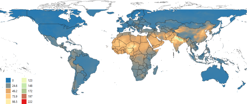
CPAT will use population weighted average PM_2.5 concentrations. In WHO databases, average concentrations are available for rural and urban areas for each country. In most countries, urban populations, in average, are exposed to higher levels of ambient PM_2.5. Figure 6.21 presents an example of urban and rural PM_2.5 for a group of countries.

Figure 6.21: Example of urban and rural weighted average concentrations

Source: World Health Organization and others (2018)

In CPAT, we also use the estimations of ambient PM_2.5 from the Global Burden of Disease Health Financing Collaborator Network (2020) study. We assume the same ratio between urban and rural concentrations levels from World Health Organization (2018) and the overall concentrations from Global Burden of Disease Health Financing Collaborator Network (2020). Figure 6.22 presents the gridded values for ambient PM_2.5 in 2019.

Figure 6.22: Gridded mean of PM_2.5, year 2019

Source: Own elaboration, based on Institute for Health Metrics and Evaluation (IHME) (2020) data

6.6.4.2 Household PM_2.5 Exposure data

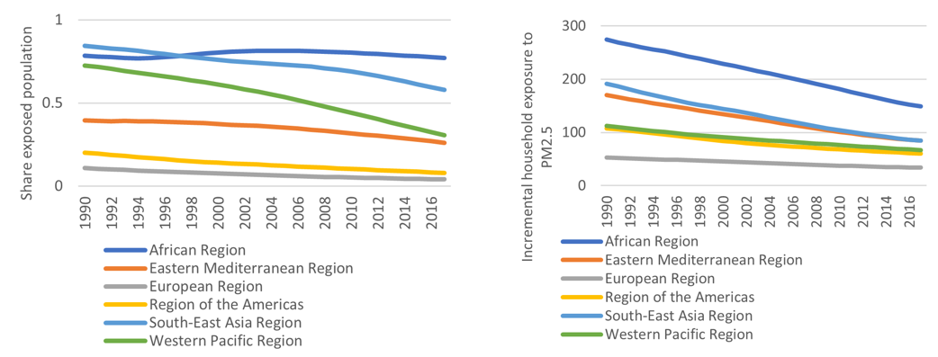
As we mentioned before, in CPAT we estimate jointly the impacts of ambient and household pollution. To do so, we need to know the share of the population exposed to household pollution and the exposure level to household PM_2.5. We again draw upon data from the Global Burden of Disease Health Financing Collaborator Network (2020) study.

The left panel in Figure 6.23 shows the estimated evolution in the share of the population exposed to household pollution in time, while the right panel presents the exposure level, in addition to the OAP exposure, for the World Bank regions. For the baseline scenario, we assume that the share of the population exposed, and the exposure level will be constant in time, and equal to the estimated value for 2019.

Figure 6.23: Share of the population (left) and level of additional population (right) exposed to households air pollution

Source: IHME/GBD, provided by Michel Brauer

6.6.4.3 Ozone Exposure data

As mentioned before, we use the seasonal 8 hours maximum daily value to estimate the health effects of ambient ozone pollution. Figure 6.24 presents the gridded concentrations estimated for 2019.

Figure 6.24: Gridded concentrations of O3, year 2019 (6mDMA8h)

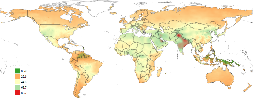
Source: Own elaboration, based on data provided by Michael Brauer

6.6.5 Leakage to biomass

Carbon pricing to formal fuels could potentially lead to an increase in the use of solid fuels²⁶ for cooking. This is called a “leakage” effect and could increase both household and ambient pollution. Figure 6.25 illustrates the carbon pricing effects on fuels consumption.

Figure 6.25: Illustration of the impact on carbon pricing in the consumption of fuels

Source: Own elaboration

The demand for fuels, including the demand for biomass for cooking is calculated in the Mitigation tab in CPAT. For details on energy demand calculations, please refer to the Mitigation tab documentation.

As illustrated in Figure 6.25, the leakage into informal fuels could increase the proportion of households exposed to HAP, the level of exposure to HAP and OAP. The assumption for OAP is that 100% of indoor emissions are eventually incorporated into ambient air (Chafe et al. (2014)). These ambient emissions are converted into ambient pollution using the methodology selected by the user, as described in Section 6.5.

Regarding the indoors effect of solid fuel use, the total leakage is divided in a fraction that increases the proportion of households and a fraction that increases the level of household pollution.

In CPAT, the defaults assumptions are that 50% of the increase in informal fuels consumption goes to additional household consuming solid fuels and 50% to increased consumption within households that were already using solid fuels.

In many countries is estimated that 90% of households or more use solid fuels for cooking. To make sure that the final proportion of households that uses solid fuels for cooking, after leakage is considered, is less than 100% (or another maximum value defined by the user), we adjust the fraction of the leakage that goes into the proportion of households. Equation 6.62 corresponds to the final proportion of households that uses solid fuels for cooking before adjustments. Equation 6.63 is the adjusted fraction in case the new share of households using solid fuels is higher than the maximum defined. Equation 6.64 is the final proportion of households using solid fuels for cooking.

\[\text{ProportionHH}_{\text{carbon\ price}} = \text{ProportionHH}_{\text{baseline}}*(1 + Leakage*F_{\text{pro}p_{\text{HH}}}) \tag{6.62}\]

\[{F\_ prop\_ HH}_{\text{adjusted}} = \left( \frac{\text{MaxPropHH}}{\text{ProportionHH}_{\text{baseline}}} - 1 \right)*\frac{1}{\text{Leakage}} \tag{6.63}\]

\[F\_ prop\_ HH = \left\{ \begin{matrix} \text{if }\text{ProportionHH}_{\text{carbon price}} > Max\ then{\ F\_ prop\_ HH}_{\text{adjusted}} \\ \text{else }\text{ProportionHH}_{\text{carbon price}} \\ \end{matrix} \right.\ \tag{6.64}\]

6.6.6 Other health effects in CPAT

6.6.6.1 Post neonatal mortality (Woodruff, Parker, and Schoendorf (2006))

In CPAT, it is possible to quantify post neonatal mortality (deaths after the first month and up to 1 year of life) using Woodruff, Parker, and Schoendorf (2006). This logistic function is presented in Equation 6.65, its applied to ambient PM_2.5, to all-cause mortality and its parameters are \(\beta=0.006765865\), with \(\sigma=0.007338828\).

\[\left( 1 - \left( \frac{1}{\left( 1 - Incidence \right)*EXP\left( \beta*DeltaQ \right) + Incidence} \right) \right)*Incidence*POP \tag{6.65}\]

6.6.6.2 Depressive disorders

Another effect of ambient air pollution included in CPAT is depressive disorders. Braithwaite et al. (2019) develops a metanalysis of studies linking long-term PM exposure and depression. The author develops a log-linear exposure-response function and uses a counterfactual value of 10 µg/m3 for the UK and of 25 µg/m3 for global scenario. In the meta-analysis, the pooled odds ratio for the association between long-term PM_2.5 exposure and depression prevalence obtained was 1.102 per 10 µg/m3 (95% CI: 1.023, 1.189; p=0:011), indicating that higher PM_2.5 exposure is associated with higher odds of depression.

They treat pooled ORs as equivalent to RRs. The relative risk can be calculated according to Equation 6.66.

\[RR \approx \text{OR}_{10}*\frac{{PM2.5}_{\text{current}} - {PM2.5}_{\text{counterfactual}}}{10} \tag{6.66}\]

Where \(OR_{10}\) denotes the OR per 10 µg/m3 increment in PM_2.5 exposure.

In CPAT, the counterfactual level, \({PM2.5}_{\text{counterfactual}}\) used is 25 µg/m3.

6.7 Methods to quantify the economic impacts of air pollution

In this section we describe the economic impacts of pollution included in CPAT. The metrics included are working days lost due to pollution, output losses due to mortality and morbidity, and health expenditure. We also explain how we value averted mortality, using a transferred VSL, the time structure of averted deaths and the valuation of travel time saved (used in CPAT Transport tab).

Figure 6.26: Economic impacts, CPAT methodology overview

6.7.1 Data sources used to quantify economic impacts

Table 6.13: Summary of data sources used to quantify economic impacts of pollution

Input	Source
Absenteeism from work	OECD (2021b), World Bank (2019b)
Methodology for working days lost	Ostro (1987), Holland (2014), ECLIPSE V5a Global Emission Fields - Global Emissions (2015)
Methodology for productivity losses	Personal communications with Maureen Cropper
Labor’s share of GDP	Guerriero (2019)
Employment to population ratio, unemployment, wages, growth rate of GDP per worker	ILOs indicators
Real interest rate27	World Development Indicators, World Bank
Health expenditure methodology	Preker et al. (2016)
Data on health expenditure	Global Burden of Disease Health Financing Collaborator Network (2019b)
VSL	OECD (2012), Narain and Sall (2016), OECD (2021a) and OECD (2021b)
Time structure of averted deaths	US EPA (2013)
Travel time saved	International Road Federation (2018), Robinson, Hammitt, and O’Keeffe (2019), Tomtom’s data.

6.7.2 Working days lost

Work absenteeism has direct costs because of wage losses and replacement costs, and indirect costs in productivity, due to delayed work and possible interference with the work performed by co-workers and supervisors.

Figure 6.27: Work absenteeism due to illness

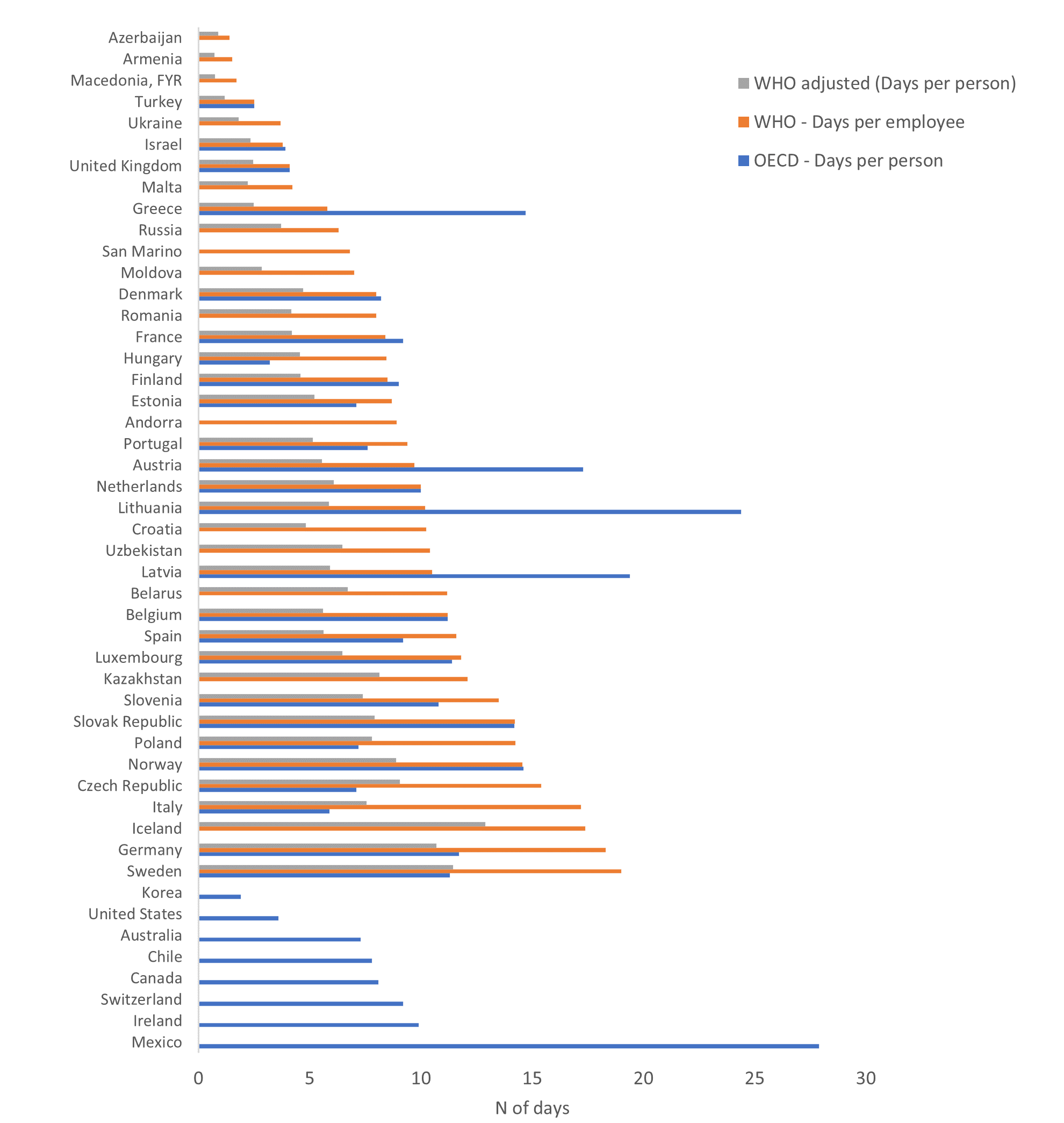
Source: OECD (2020) and WHO (2019)

In CPAT, we quantify working days lost attributed to pollution following Ostro (1987). This methodology has been implemented in more recent literature, such as Holland (2014) and Amann et al. (2017). OECD research OECD (2016) and OECD (2019) has also been based indirectly in Ostro (1987) but referencing the work from Holland (2014).

The baseline absenteeism from work due to illness data used are the OECD database “Absence from work due to illness” (OECD (2020)) that covers 46 countries²⁸ and “Absenteeism from work due to illness”²⁹ from the WHO (2019). Figure 6.27 presents the data from the observed databases.

Since not every country is covered in the databases, we adopt the following assumptions for obtaining baseline absenteeism at a country level:

• If the country in included in the OECD database, we use OECD data.

• If no OECD data is available, but WHO data includes the country, we use WHO adjusted by “employment to total population ratio, 15+” (ILO n.d.).

• If no country specific data is available, we use the average value among countries with the same income level.

• For low-income countries (that are not represented in either database), we use the average from lower middle-income countries.

To calculate the share of work absenteeism due to illness that can be attributed to ambient PM_2.5 pollution, we use the methodology from Ostro (1987). The study developed a log-linear function with \(\beta = 0.0046\) and \(\sigma_{\beta} = 0.00036\). The attributable fraction of working days lost due to pollution is calculated using Equation 6.67 and the total number of days lost due to pollution is given by Equation 6.68.

\[PAF = 1 - e^{- \beta*\mathrm{\Delta}C} \tag{6.67}\]

\[\text{WDL}_{\text{pollution}} = \text{Pop}_{15\ to\ 64}*\text{Per\ person\ WDL}_{\text{baseline}}*(1 - e^{- \beta*C\ baseline}) \tag{6.68}\]

Where \(\Delta C\) is the current level of PM_2.5 minus a reference level for PM_2.5, that is assumed to be 0 in this case.

To value the days of work lost due to pollution, we use mean monthly earnings of employees, ILOSTAT Labor statistics.

If no wage is available, the default value used is: \[Daily\ wage = \frac{GDP*\alpha}{N{^\circ}\ of\ persons\ employed}*\frac{1}{N{^\circ}\ of\ days} \tag{6.69}\]

Where \(N{^\circ}\ of\ days\ = 12*20\).

We consider working population from 15 to 64 years old, as in Amann et al. (2017).

6.7.3 Market output losses

In CPAT, we quantify market output losses using mortality and years lived with disability (YLD) attributed to pollution, following the methodology in Pandey et al. (2021). The methodology followed is presented in the following paragraphs.

Average GDP contribution by worker

Equation 6.70 presents the expected value of GDP per worker in a given year, that we will use to quantify GDP losses due to pollution.

\[W_{\text{ij}} = \left( \frac{L_{\text{ij}}}{N_{\text{ij}}} \right)\left( \frac{\text{αY}_{i}}{L_{i}} \right) \tag{6.70}\]

Where:

\(W_{ij}\): the expected value of GDP per worker for a person of age \(j\) in state \(i\).

\(\alpha\): Labor’s share of GDP

\(Y_i\): GDP

\(L_i\): number of persons who are employed

\(N_{\text{ij}}\): Population of age\(\text{\ j}\) in state \(i\)

Due to data limitations, in CPAT will compute a value \(W\) for every worker above 15+, without differentiating by age or by urban and rural areas.

For each period (year) \(p\), the expected GDP from labor per person is calculated using Equation 6.71.

\[W_{p} = \left( \frac{L_{p}}{N_{p}} \right)\left( \frac{\text{αY}_{p}}{L_{p}} \right) = \ \frac{\text{αY}_{p}}{N_{p}} \tag{6.71}\]

Loss in market and non-market output due to air pollution mortality

Losses in market and non-market output due to air pollution mortality can be estimated according to Equation 6.72.

\[{W'}_{ij2017} = \left( \frac{L_{\text{ij}}}{N_{\text{ij}}} \right)\left( \frac{\text{αY}_{i}}{L_{i}} \right) + hp\left( 1 - \frac{L_{\text{ij}}}{N_{\text{ij}}} \right)\left( \frac{\text{αY}_{i}}{L_{i}} \right) \tag{6.72}\]

Where \(hp\) represents household production. In CPAT, due to data limitations, we will only include losses in market output.

The present value of the forgone output associated to a premature death is calculated according to Equation 6.73.

\[\text{PV}_{\text{ij}} = \sum_{a = j}^{84}\pi_{ij,t}\left\lbrack \left( \frac{L_{\text{it}}}{N_{\text{it}}} \right)\left( \frac{\text{αY}_{i}}{L_{i}} \right) + hp\left( 1 - \frac{L_{\text{it}}}{N_{\text{it}}} \right)\left( \frac{\text{αY}_{i}}{L_{i}} \right) \right\rbrack\left( \frac{1 + g}{1 + r} \right)^{t - j} \tag{6.73}\]

Where:

\(\text{PV}_{\text{ij}}\): present discounted value of lost market and non-market output for a person of age \(j\) in state \(i\) who dies in a certain year

\(g\): growth rate of GDP per worker

\(\Pi_{ij,t}\) is the probability that a person of age \(j\) in state \(i\) survives to age \(t\)

\(r\): discount rate

In CPAT, \(W_{ij,t} = W_{p}\) (does not change by age or within countries). We will also consider only deaths up to 64, neglecting work force above 65. These assumptions, together with assuming \(\text{hp}=0\), allow us to rewrite Equation 6.73 as Equation 6.74.

\[\text{PV}_{j} = W*\sum_{t = j}^{64}\pi_{j,t}*\left( \frac{1 + g}{1 + r} \right)^{t - j} \tag{6.74}\]

Rewriting Equation 6.74, we obtain:

\[\text{PV}_{j}/W = \sum_{t = j}^{64}\pi_{j,t}*\left( \frac{1 + g}{1 + r} \right)^{t - j} \tag{6.75}\]

The total output lost due to air pollution attributed mortality is obtained using Equation 6.76.

\[TotalOutputLost = \sum_{j}^{}{\text{PV}_{\text{ij}}D_{\text{ij}}} \tag{6.76}\]

With \(D_{\text{ij}}\) the number of deaths attributed to air pollution in state \(i\) of age \(j\).

GDP loss due to air pollution morbidity

In CPAT, we estimate the years lived with disability due to pollution (see Section 6.6.3.2). We value those years, in which people in working age are not able to work, or the output loss associated with morbidity using Equation 6.77.

\[M\text{ij}\ = \ \ Wij*\text{YLD}\text{ij} \tag{6.77}\]

Table 6.14 presents the data sources used for the different productivity parameters needed to quantify output losses.

Table 6.14: Parameters for productivity

Parameter		Data sources
\(\alpha\)	Labor’s share of GDP	Guerriero (2019), includes 117 countries. If there isn’t data available for a country, we use the world’s average labor share of GDP, of 65%.
\(Y_i\)	GDP	World Bank national accounts data, and OECD National Accounts data files
\(\frac{L_{\text{it}}}{N_{\text{it}}}\)	Labour to population	Employment to population ratio, 15+, total (%) (modeled ILO estimate), International Labour Organization, ILOSTAT database. Data retrieved in April 2019
\(L_{it}\)	Number or persons that are employed	\[L=LaborForcetotal*(1 − unemployment)\] Labor force30 derived using data from International Labour Organization, ILOSTAT database and World Bank population estimates. Labor data retrieved in April 2019. Unemployment from International Labour Organization, ILOSTAT database. Data retrieved in April 2019.
\(hp\)	Household production	Not included in CPAT
\(\Pi_{it,t}\)	Probability of survival	The probability of survival is the probability that an individual would have survived to each future year of his working life. The probability of death31 is obtained from Global Burden of Disease Collaborative Network (2018) for every country and age group. The probability of survival up to 64 years is calculated as follows: \[\pi_{j} = \prod_{j}^{64}{(1 - \text{Prob\ of\ death}_{j})}\]
\(g\)	growth rate of GDP per worker	ILO indicators32, up to 2023: - SDG indicator 8.2.1 - Annual growth rate of output per worker (GDP constant 2010 USD) (%). After 2023, we assume a growth rate equal to the rate in 2023.
\(r\)	Discount rate	CPAT allows the user to select among 3 options: i) Use the real interest rate for the country, ii) Using a 3% discount rate, as recommended in Robinson, Hammitt, and O’Keeffe (2019), iii) Input manually a discount rate. In case the user selects the first option, r will be the real interest rate33 (%) from the International Monetary Fund, International Financial Statistics and data files using World Bank data on the GDP deflator34. That data covers 127 countries. Data is available up to 2018. After 2018, it’s assumed an interest rate equal to the average of the rates between 2014 and 2018.

6.7.3.1 CPAT operationalization

From the GBD Results Tool, we obtained deaths probabilities for five-years buckets. For instance, we know the probability of dying between 25 to 29 years old (\(d_{25,29}\)). The probability \(d_{25,29}\) is equal to the sum of the probability of dying at 25, at 26, at 27, at 28 and at 29 years old, as shown in Equation 6.78.

\[d_{25,29} = d_{25} + d_{26} + d_{27} + d_{28} + d_{29} \tag{6.78}\]

For simplicity and to keep the file size at a reasonable level, we will assume that the probability of dying at every age contained in each bucket is the same, and equal to the bucket dying probability divided by 5, as presented in Equation 6.79.

\[d_{25} = d_{26} = d_{27} = d_{28} = d_{29} = \frac{d_{25,29}}{5} \tag{6.79}\]

The survival probability for each age inside each age-bucket is presented in Equation 6.80.

\[\pi_{25,29} = \left( 1 - \frac{d_{25,29}}{5} \right) = \pi_{25} = \pi_{26} = \pi_{27} = \pi_{28} = \pi_{29} \tag{6.80}\]

To implement Equation 6.75, let’s do \(\left( \frac{1 + g}{1 + r} \right) = a\). Then, Equation 6.75 operationalized for 5 years bucket in CPAT is presented in Equation 6.81.

\[\frac{\text{PV}_{25 - 29}}{W} = \pi_{25,29}*\sum_{k = 0}^{2}a^{k} + \pi_{25,34}*\sum_{k = 3}^{7}{a^{k} + \ldots + \pi_{25,64}*\sum_{k = 43}^{47}a^{k}} \tag{6.81}\]

Where \(k = t - j\)

To solve the sums inside Equation 6.81, we can apply the following formula:

\[\sum_{k = 0}^{n}{a^{k} = \frac{1 - a^{n + 1}}{1 - a}} \tag{6.82}\]

Equation 6.82 can be used to solve the sum terms that start in \(k≠0\), as shown in Equation 6.83.

\[\sum_{k = m}^{n}{a^{k} = \sum_{k = 0}^{n}a^{k} - \sum_{k = 0}^{m}a^{k} = \frac{1 - a^{n + 1}}{1 - a} - \frac{1 - a^{m + 1}}{1 - a}} \tag{6.83}\]

6.7.4 Health expenditure

In CPAT, we use total expected health expenditure from 2017 to 2050 from the IHME (Global Burden of Disease Health Financing Collaborator Network (2019a)).

We follow Preker et al. (2016) to estimate the share of total health expenditure than can be attributed to pollution. The assumption is a constant expenditure per DALY (Disability adjusted life years).

In CPAT, we calculate the share of the total burden of disease that’s attributed to the 6 main causes related to pollution, using data from the GBD Results Tool (Institute for Health Metrics and Evaluation (IHME) (2020)). The share of the burden of disease for disease \(d\), country \(c\) and year \(t\), \(\% BoD_{d,c,t}\), is calculated according to Equation 6.84.

\[\% BoD_{d,c,t} = \frac{\text{DALY}s_{d,c,t}}{\text{TotalDALY}s_{c,t}} \tag{6.84}\]

The total health expenditure attributed to pollution \(\text{HEAP}\) can be calculated using Equation 6.85.

\[\text{HEAP}_{c,t} = \sum_{d}^{}{\% BoD_{d,c,t}*PAF_{d,t}*THE_{c,t}} \tag{6.85}\]

Where:

\(\text{PAF}_{d,t}\): population attributable fraction for disease \(d\) in year \(t\)

\(\text{THE}_{c,t}\): Total health expenditure for country \(t\) in year \(t\)

\(\text{DALY}s_{d,c,t}\): Disability adjusted life years, for disease \(d\), country \(c\) and year \(t\)

In CPAT, we distribute health expenditure between government, prepaid private, out-of-pocket and development assistance for health using IHME estimations for 2019 (Global Burden of Disease Health Financing Collaborator Network (2019a)).

6.7.5 Value of the statistical life

In CPAT, we value averted mortality using the value of the statistical life or VSL. It’s important to notice that the VSL does not represent the value of individual lives. Rather, the VSL is a measure of the rate at which individuals are willing to exchange money to reduce small risks of death within a certain period of time. This concept is used in benefit-cost analyses, and we include it in CPAT to assign a monetary value to averted mortality due to a carbon price policy.

The VSL can be transferred following the methodology from OECD (2012) and Narain and Sall (2016), according to Equation 6.86.

\[VSL_{c} = VSL_{OECD,2005}*\left( \frac{Y_{c}}{Y_{OECD,2005}} \right)^{b}*\left( 1 + \%\mathrm{\Delta}P + \%\mathrm{\Delta}Y \right)^{b} \tag{6.86}\]

Where:

\(c\): Country to which VSL in being transferred to.

\(\text{VSL}_{OECD,2005}\): Median VSL in OECD countries in 2005, in 2005 $USD PPP

\(Y\): GDP per capita in PPP

\(b\): Income elasticity for VSL in country \(c\)

\(\%\mathrm{\Delta}Y\): Income growth after 2005

\(\%\mathrm{\Delta}P\): inflation according to consumer price index

In CPAT, we first transform OECD VSL from 2005 USD PPP to 2011 PPP, using Equation 6.87.

\[VSL_{OECD,\ t,2011PPP} = VSL_{OECD,2005}*\left( \frac{Y_{OECD,t}}{Y_{OECD,2005}} \right)^{0.8}*\left( 1 + \%\mathrm{\Delta}P_{2005,2011} \right)^{0.8} \tag{6.87}\]

Secondly, we transfer the OECD VSL from 2014 (in 2011 USD PPP) to the destiny country, according to Equation 6.88.

\[VSL_{OECD,\ 2014} = VSL_{OECD,\ 2014}*\left( \frac{Y_{c,2014}}{Y_{OECD,2014}} \right)^{b} \tag{6.88}\]

Thirdly, we project VSL in time using projected GDP per capita for country \(c\), according to Equation 6.89.

\[VSL_{c,\ t} = VSL_{c,2014}*\left( \frac{Y_{c,t}}{Y_{c,\ 2014}} \right)^{b} \tag{6.89}\]

Finally, we convert the VSL from 2011 dollars to dollars in the “Results Year” (equal to 2019), using the 2019 price deflator for the country of destiny.

In CPAT, income elasticity is assumed equal to 0.8 for high-income countries and 1.2 for middle and low-income countries. The user can also input manually a different elasticity and a different VSL value in the Advanced tab of CPAT.

Table 6.15 and Table 6.16 present the values assumed to transfer the VSL from OECD countries.

Table 6.15: Assumptions and data sources for VSL transfer

Variable	Assumption	Source
\(VSL_{OECD, 2005}\)	3 million USD in 2005, in 2005 PPP dollars	OECD (2012), Table 6.1
\(b\)	0.8 for high income countries and 1.2 for middle and low-income countries	Narain and Sall (2016)

Table 6.16: Consumer price index and GDP per capita, OECD countries

Year	CPI OECD	GDP per head of population OECD (2011 $US PPP)
2005	82.0	35,407.8
2006	84.1	36,248.1
2007	86.2	36,921.0
2008	89.4	36,738.5
2009	89.9	35,198.6
2010	91.5	36,011.9
2011	94.1	36,554.1
2012	96.2	36,813.9
2013	97.7	37,130.2
2014	99.4	37,696.5
2015	100.0	38,413.8
2016	101.1	38,859.1
2017	103.4	39,589.2

Source: OECD (2021a) and OECD (2021b)

6.7.6 Time Structure of averted deaths

When quantifying and valuing premature mortality, it is often assumed that there is a “cessation lag,” or time distribution of averted mortality after a reduction in exposure (US EPA (2013)). The time structure we selected assumes that 30% of mortality reductions occur during the first year, 50% occurs over years 2 to 5 and 20% over years 6 to 20, after the PM_2.5 reduction takes place.

When valuing averted mortality using the value of statistical life (VSL), it is possible to calculate the present value of the benefit from reduced premature deaths by applying the discount rate to the number of deaths themselves and then multiplying by the VSL. In CPAT, the user can select the discount rate among 3 options: i) a discount rate of 3%, consistent with the recommendation in Robinson et al. (2019); ii) a discount rate that represent the interest rate paid by the country’s government and iii) a manual input of discount rate. When using a 3% discount rate, the present value of premature deaths reduced is 0.906 times the number of undiscounted premature averted deaths. When using a higher discount rate, for example a rate of 8%, the factor is reduced to 0.798 (see Table 6.17).

Table 6.17: Time distribution of averted premature deaths

		3% discount rate	8% discount rate
	Deaths distribution in time	Time discount factor	Fraction deaths*time discount factor	Time discount factor	Fraction deaths*time discount factor
Year 0	30.0%	1.00	0.300	1.00	0.300
Year 1	12.5%	0.97	0.121	0.93	0.116
Year 2	12.5%	0.94	0.118	0.86	0.107
Year 3	12.5%	0.92	0.114	0.79	0.099
Year 4	12.5%	0.89	0.111	0.74	0.092
Year 5	1.3%	0.86	0.012	0.68	0.009
Year 6	1.3%	0.84	0.011	0.63	0.008
Year 7	1.3%	0.81	0.011	0.58	0.008
Year 8	1.3%	0.79	0.011	0.54	0.007
Year 9	1.3%	0.77	0.010	0.50	0.007
Year 10	1.3%	0.74	0.010	0.46	0.006
Year 11	1.3%	0.72	0.010	0.43	0.006
Year 12	1.3%	0.70	0.009	0.40	0.005
Year 13	1.3%	0.68	0.009	0.37	0.005
Year 14	1.3%	0.66	0.009	0.34	0.005
Year 15	1.3%	0.64	0.009	0.32	0.004
Year 16	1.3%	0.62	0.008	0.29	0.004
Year 17	1.3%	0.61	0.008	0.27	0.004
Year 18	1.3%	0.59	0.008	0.25	0.003
Year 19	1.3%	0.57	0.008	0.23	0.003
Total Lag factor	0.906		0.798

Source: Own elaboration Note: \(Time\ discount\ factor\ = 1/(1 + r)^{(t - t0)}\)

6.7.7 Travel time saved

Excess travel time is one of the consequences of road congestion. In CPAT, we estimate excess travel time, increased road damage, increased injuries, and additional vehicle operating costs attributable to congestion. The methodology used is described in the document Road Transport documentation. Here we only describe the methodology used to quantify changes in travel time, in time units, with respect to free a flow condition.

We estimate travel time per vehicle-kilometer in free flow and in congested conditions for 416 cities in 57 countries, using TomTom data (see Equation 6.91 and Equation 6.90). The time domain used is “All Days Full Day”.

Congestion travel time per vehicle-kilometer, \(CongestionTT\), is calculated using Equation 6.90.

\[\text{CongestionT}T_{2019}\lbrack min/vehkm\rbrack = \frac{\text{AccumulatedTravelTim}e_{2019}\ \lbrack min\rbrack}{\text{TotalVeh}\text{KM}_{2019}\lbrack vehkm\rbrack} \tag{6.90}\]

\(\text{TotalVehicleKM}\) corresponds to the multiplication of the number of vehicles and the average distance traveled and is reported in the TomTom database.

The travel time per vehicle-kilometer under free flow conditions is calculated using Equation 6.91.

\[FreeFlowTT\lbrack\frac{\min}{\text{vehkm}}\rbrack = \frac{\text{CongestionT}T_{2019}\ \lbrack\frac{\min}{\text{vehkm}}\rbrack}{(1 + \frac{CI_{2019}}{100})} \tag{6.91}\]

Where \(\text{CI}\) is the average congestion index in 2019.

We estimate vehicle-kilometers traveled per capita using total vehicle-kilometers from the World Road Statistics data (International Road Federation (2018)) and countries total population (World Bank (2019b)). For those countries not included in the WRS database, we assume the average vehicle-kilometers traveled per capita between the regional mean and the income level mean.

Using vehicle-kilometers traveled per capita, together with the congestion index \(CI\) and the free flow travel time, we can estimate total travel time each year \(t\), in time units, using Equation 6.92.

\[\text{Travel time}_{t} = \left( 1 + \frac{CI_{t}}{100} \right)*FreeFlowTT\left\lbrack \frac{\min}{\text{vehkm}} \right\rbrack*VehKm\ per\ capita\left\lbrack \frac{\text{vehkm}}{\text{year}} \right\rbrack*UrbanPopulation_{15 + ,t} \tag{6.92}\]

In CPAT, there are estimations for the congestion index for each year, under the baseline scenario and a carbon price scenario. Using the Equation 6.92, we can quantify travel time for each year under each scenario. Time savings attributed to a carbon price are equal travel time in the baseline minus travel time in the carbon price scenario.

We value those time savings following Robinson et al. (2019). We value travel time at a rate of 50% the after-tax wage rate. We use gross earnings³⁵ data from ILO and then we apply a factor to estimate after-tax wages. The factor used for OECD countries is the “average income tax rate as % of gross wage earnings”. For other countries, we use the average factor from OECD countries, equal to 16%. When we value travel time savings, we do so by considering only the population above 15 years old, since younger population does not participate in the labor market.

Some implied assumptions: We assume that free flow travel time and vehicle-kilometers traveled per capita are constant in time. Vehicle-kilometers traveled are the same across the population, regardless of age or other considerations. Tomtom’s data is representative of vehicles not using their devices.

6.7.8 Value of morbidity using years lived with disabilities (YLDs)

Another approach to value morbidity in CPAT in based on a method proposed in Bank (2022). Under this method, we convert YLDs to ‘annual disease days’ \(M\) and we value them using a fraction of a country’s daily wage.

First, annual disease days are calculated from YLDs, for each country as:

\[M = \ \sum_{c = 1}^{n}{YLD_{c}*\frac{365}{DW_{c}}} \tag{6.93}\]

Where:

\(YLD_{c}\): years lost to disease \(c\)

\(DW_{c}\) : Average disability weight of disease \(c\) attributed to PM_2.5

The cost of a day lived with a disease \(c\), \(c_{c}\), is calculated a fraction of the daily wage \(w\) (in each country), as presented in Equation 6.94. The term D corresponds is set at 0.4, and is associated to the disability weight of a severe condition, with severely restricted work and leisure activity and a substantial medical cost.

\[c_{c} = w*\frac{DW_{c}}{D} \tag{6.94}\]

The average daily wage, \(w\), was calculated using the methodology explained in Section 6.7.3.

Finally, the cost of morbidity is calculated as the multiplication of annual disease days and the cost of each day lived with disease.

\[Cost\ of\ Morbidity = \ \sum_{i = 1}^{n}{c_{c}*M} \tag{6.95}\]

Using this method to value morbidity attributed to air pollution, we calculate the share of morbidity costs as a share of mortality costs.

6.7.9 Air pollution externalities per unit of fuel

The health impacts attributed to air pollution are calculated jointly for ambient and household pollution (see Section 6.6.3), following the methodology from Global Burden of Disease Health Financing Collaborator Network (2020). Although the health impacts are estimated jointly, we compute an average externally cost per unit of fossil fuel burnt, which affects only ambient pollution.

After the health impacts have already been quantified, the air pollution externality computation is made as follows:

1. We compute the average ambient air pollution attributed mortality per µg/m3 of PM_2.5 as total mortality attributed to ambient PM_2.5 in a certain year (referred to as “attributable burden” in previous chapters) divided by the total ambient PM_2.5 that year.

2. Using the emission factor (for each fuel and sector, for each country) and the emissions-to-concentrations model selected, we compute the ambient PM_2.5 contributed by one unit of fuel used (in µg/m3 of PM_2.5 per ktoe).

3. We multiply the average ambient air pollution attributed mortality per µg/m3 (step 1) with the ambient PM_2.5 contributed by one unit of fuel used (step 2), obtaining the number of attributed deaths by unit of fuel used (deaths/ktoe).

4. We multiply the metric calculated in step 3 with the VSL for the corresponding year and country, obtaining the externality value in dollars per ktoe. We add to this number morbidity costs (for ambient air pollution), according to the methodology described in Section 6.7.8.

5. We convert energy units to express the externality in a commonly used metric for each fuel, considering the relevant calorific values in each country and fuels densities when needed. For instance, for gasoline, the externality is expressed as US$ per liter, while, for coal, the externality is expressed as US$ per GJ.

6.8 Validation: comparison with other models

6.8.1 Health impacts of pollution

In the following figures, we compare CPAT results with external models. Green dots represent CPAT results, and the blue line represents the results from the external model. When the green dots are above the blue line (45 degrees line), CPAT estimates are higher, and when the green dots are below the line, CPAT estimates are lower.

Figure 6.28: CPAT estimation of ambient PM_2.5 air pollution death rates versus GBD2019 estimates

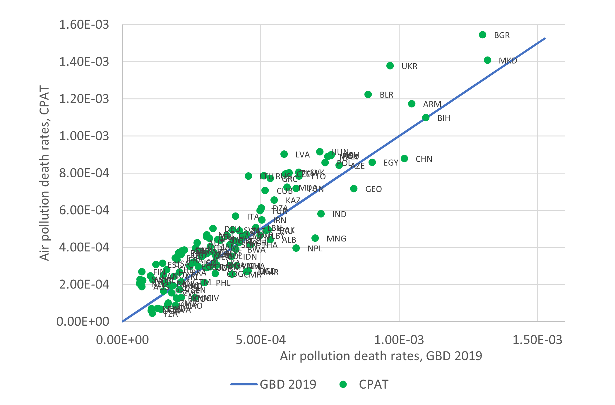
Source: CPAT results and Global Burden of Disease Health Financing Collaborator Network (2020)

6.8.2 Emissions

Figure 6.29: PM_2.5 emissions in the transport sector, CPAT 2020 versus EDGAR 2015 and IIASA 2020

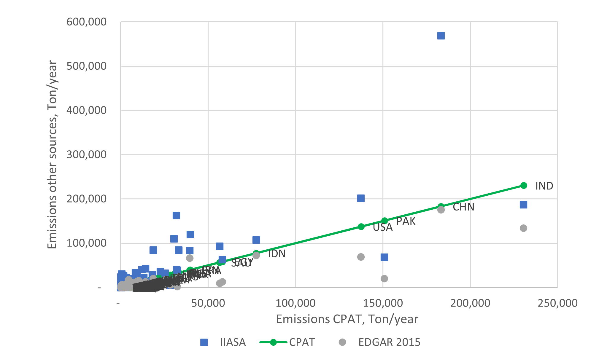
Source: CPAT results, European Environment Agency (2020) and ECLIPSE V5a Global Emission Fields - Global Emissions (2015)

Figure 6.30: PM_2.5 emissions in the power sector, CPAT 2020 versus EDGAR 2015 and IIASA 2020

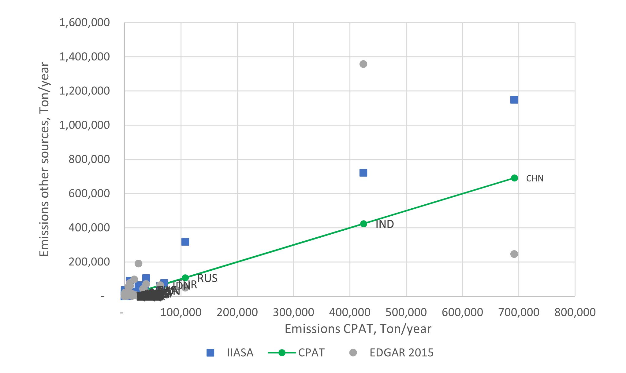
Source: CPAT results, European Environment Agency (2020) and ECLIPSE V5a Global Emission Fields - Global Emissions (2015)

6.8.3 Concentrations: share of fossil fuels on ambient PM_2.5

Figure 6.31: Comparison of the share of fossil fuels contribution to ambient PM_2.5 from Vohra et al. (2021) and CPAT “Avg. iF and LS FASST” (Option 6 of this documentation)

Source: Own elaboration. Note: Vohra et al. (2021) share of FF contribution to ambient PM_2.5 if higher than in CPAT for 61% of countries

Figure 6.32: Comparison of the share of fossil fuels contribution to ambient PM_2.5 from Vohra et al. (2021) and CPAT “Machine Learning” (Option 5 in this documentation)

Source: Own elaboration. Note: Vohra et al. (2021) share of FF contribution to ambient PM_2.5 if higher than in CPAT for 55% of countries

Figure 6.33: Comparison of the share of fossil fuels contribution to ambient PM_2.5 from Vohra et al. (2021) and CPAT “Local Study-FASST” (Option 2 in this documentation)

Source: Own elaboration. Note: Vohra et al. (2021) share of FF contribution to ambient PM_2.5 if higher than in CPAT for 44% of countries

Figure 6.34: Comparison of the share of fossil fuels contribution to ambient PM_2.5 from Vohra et al. (2021) and CPAT “Intake fractions” (Option 4 in this documentation)

Figure 6.35: Modeled contribution of fossil fuels to ambient PM_2.5. Vohra et al. (2021) versus CPAT (average among 6 options to relate emissions and concentrations)

6.8.4 Externalities from pollution

Figure 6.36: Comparison among CPAT results and Korteland (2022)

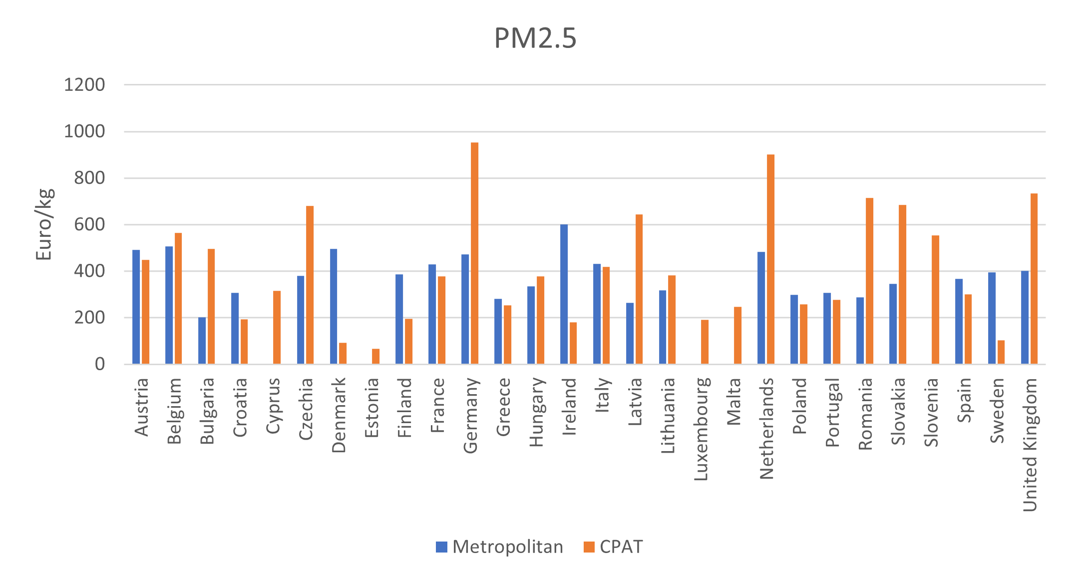
6.9 Caveats

The health impacts are calculated using global relative risk functions and global data bases regarding exposure to pollution, baseline incidence and others. Global databases are constructed using country level databases, but in many cases, they are adjusted and standardized. This may lead to differences among the data used in CPAT and local databases. If differences among CPAT and local data is an issue, an advanced Excel user could modify any inputs in CPAT, since the spreadsheet is open, but this would require a deep understanding of the tool.

Another issue to be aware of is the national and yearly scope of CPAT. This can be a limitation of CPAT analysis because the dynamics of air pollution can vary widely inside countries and throughout the year. CPAT intends to represent population weighted average air pollution for average pollution during a calendar year.

Another caveat is the uncertainty on the calculation of emissions, the relationship between emissions and ambient concentration, the health impacts and the economic values used to monetize the impacts of pollution. CPAT at the time is providing a central estimate for all calculations, without indicating uncertainty on estimations. This caveat could be partially addressed by using the “MT tool” (described in the user guide) to do a sensitivity analysis on the assumptions used.

It is important to consider that, even though CPAT performs well when compared to other more complex models, this does not guarantee that CPAT results will always be consistent with other more advance models. We have compared baseline estimates with external global sources, to make sure that we represent the baseline properly. Many checks have been performed in the Mitigation module too, which results drive the air pollution results. These checks do not guarantee that the policy impacts obtained using CPAT will be similar to those obtained from other more complex models. Further checks will need to be performed in a policy/country-specific context. CPAT allows the user to change assumptions and inputs, such that the tool can be adjusted properly when needed.

Overall, the results from the air pollution in CPAT are conservative in the sense the results are likely underestimating the health impacts of a climate policy. This is the case in big part because the default configuration of the air pollution variables yields conservative contribution from fossil fuels to air pollution. The user can change the predefined options and calibrate the tool to make the results consistent with other sources of information available.

6.10 Appendices

6.10.1 CPAT codes, Air Pollution tab.

Air pollution tab codes:

Variables	Code	Description
Series	paf	Population attributable fraction
	rr	Relative risk
	em	Emission
	con	Concentration
	pop	Population
	ph	Proportion of population using solid fuels for cooking and thus exposed to household pollution
	inc	Incidence proportion
	dth	Deaths
	Yll	Years of life lost
	Yld	Years lived with disabilities
	daly	Disability-adjusted life years
	mrf	Multiple risk factor (for COPD)
	src	Source-receptor coefficients from FASST
Pollutants	Pm2	PM2.5 (concentration)
	O3	Ozone (concentration)
Risks	Oap	Ambient or outdoors pollution
	Hap	Household air pollution
	Hop	Ambient + household pollution
	bur	Ambient pollution, using Burnett et al 2018
Diseases	Lri	Lower respiratory diseases
	Lun	Tracheal and lung cancer
	Cop	Chronic obstructive pulmonary disease
	Dme	Diabetes mellitus type II
	Str	Stroke
	Ihd	Ischemic heart disease
	dep	Depressive disorders
	dne	Diseases for neonates: Sudden infant death syndrome, Diarrheal diseases, Lower respiratory infections, Upper respiratory infections, Otitis media, Meningitis, Neonatal disorders, Encephalitis
Age	All
	25 to 64
	65+
Area	Urb	Urban areas
	rur	Rural areas
	all	Urban and rural areas
Others	Conc. pm2.fas.usr.	Concentration by sector according to user’s information, with precursors weight calculated using FASST
	conc.pm2.fas.lst	Concentration by sector according to local study, with precursors weight calculated using FASST
	Conc.pm2.cm.lst	Concentration by sector according to local study, with precursors weight calculated using CM (from Apte or Fantke)
	eln	Elastic net model to relate emissions and concentrations

6.10.2 Relative Risk IER GBD 2019

Table 6.18: IER GBD 2019 for lung cancer, COPD, diabetes mellitus type II, LRI, low birthweight and pre-term birth

PM2.5 (µg/m³)	Tracheal, bronchus, and lung cancer	Chronic obstructive pulmonary disease	Diabetes mellitus type 2	Lower respiratory infections	Low birthweight	preterm birth
600	1.76	5.19	1.56	2.48	1.3281	1.6024
500	1.73	4.54	1.54	2.44	1.2870	1.5498
400	1.70	3.89	1.52	2.40	1.2459	1.4973
300	1.67	3.24	1.50	2.34	1.2049	1.4448
200	1.64	2.59	1.48	2.07	1.1638	1.3922
150	1.62	2.27	1.47	1.88	1.1432	1.3659
120	1.61	2.05	1.46	1.74	1.1309	1.3502
90	1.57	1.83	1.46	1.59	1.1186	1.3336
75	1.54	1.71	1.45	1.51	1.1124	1.3120
60	1.49	1.58	1.45	1.42	1.1062	1.2722
45	1.42	1.45	1.44	1.33	1.1001	1.2201
30	1.32	1.31	1.40	1.22	1.0922	1.1603
25	1.28	1.26	1.37	1.19	1.0875	1.1388
20	1.24	1.21	1.33	1.15	1.0809	1.1161
15	1.19	1.16	1.28	1.12	1.0721	1.0916
10	1.13	1.11	1.21	1.08	1.0603	1.0645
5	1.07	1.06	1.11	1.04	1.0404	1.0342
0	1.00	1.00	1.00	1.00	1.0000	1.0000

Source: Own elaboration based on Global Burden of Disease Health Financing Collaborator Network (2020)

Table 6.19: IER GBD 2019 for Ischemic heart disease and stroke

	PM2.5 (µg/m³)	25-29	30-34	35-39	40-44	45-49	50-54	55-59	60-64	65-69	70-74	75-79	80-84	85-89	90-94	95+
Ischemic heart disease	600	2.83	2.69	2.53	2.41	2.29	2.14	2.06	1.93	1.83	1.76	1.64	1.53	1.47	1.36	1.27
	500	2.79	2.65	2.49	2.37	2.25	2.11	2.02	1.89	1.79	1.72	1.61	1.50	1.44	1.34	1.25
	400	2.75	2.61	2.45	2.33	2.20	2.07	1.98	1.86	1.76	1.68	1.57	1.48	1.41	1.32	1.24
	300	2.71	2.57	2.41	2.29	2.16	2.03	1.93	1.82	1.72	1.64	1.54	1.45	1.38	1.29	1.22
	200	2.67	2.52	2.37	2.24	2.12	1.99	1.89	1.78	1.68	1.60	1.50	1.42	1.35	1.27	1.20
	150	2.65	2.50	2.35	2.22	2.10	1.97	1.87	1.76	1.66	1.58	1.49	1.40	1.33	1.26	1.19
	120	2.64	2.49	2.34	2.21	2.08	1.96	1.86	1.75	1.65	1.57	1.48	1.40	1.32	1.25	1.18
	90	2.61	2.47	2.31	2.19	2.06	1.94	1.84	1.73	1.64	1.55	1.46	1.38	1.31	1.24	1.18
	75	2.53	2.39	2.24	2.13	2.01	1.90	1.80	1.69	1.61	1.52	1.44	1.37	1.30	1.23	1.17
	60	2.37	2.24	2.12	2.01	1.91	1.81	1.73	1.63	1.55	1.48	1.41	1.34	1.27	1.21	1.16
	45	2.16	2.05	1.95	1.86	1.78	1.70	1.62	1.54	1.48	1.41	1.35	1.29	1.24	1.19	1.14
	30	1.88	1.80	1.72	1.66	1.60	1.54	1.48	1.42	1.37	1.32	1.28	1.23	1.19	1.15	1.11
	25	1.76	1.69	1.63	1.58	1.52	1.47	1.42	1.36	1.33	1.28	1.24	1.20	1.17	1.13	1.10
	20	1.64	1.58	1.53	1.49	1.44	1.40	1.36	1.31	1.27	1.24	1.20	1.17	1.14	1.11	1.08
	15	1.50	1.46	1.42	1.38	1.35	1.32	1.28	1.24	1.22	1.19	1.16	1.14	1.11	1.09	1.07
	10	1.35	1.32	1.29	1.27	1.24	1.22	1.20	1.17	1.15	1.13	1.11	1.10	1.08	1.06	1.05
	5	1.18	1.17	1.15	1.14	1.13	1.12	1.11	1.09	1.08	1.07	1.06	1.05	1.04	1.03	1.02
	0	1.00	1.00	1.00	1.00	1.00	1.00	1.00	1.00	1.00	1.00	1.00	1.00	1.00	1.00	1.00
Stroke	600	3.53	3.31	3.08	2.88	2.73	2.52	2.37	2.21	2.09	1.94	1.82	1.73	1.63	1.54	1.43
	500	3.49	3.27	3.04	2.84	2.69	2.48	2.33	2.17	2.05	1.90	1.78	1.69	1.59	1.49	1.39
	400	3.44	3.23	3.00	2.80	2.65	2.44	2.29	2.13	2.01	1.87	1.74	1.65	1.55	1.45	1.35
	300	3.40	3.19	2.96	2.76	2.61	2.41	2.25	2.09	1.97	1.83	1.71	1.61	1.50	1.41	1.31
	200	3.36	3.15	2.92	2.72	2.56	2.37	2.21	2.06	1.93	1.79	1.67	1.57	1.46	1.37	1.27
	150	3.33	3.13	2.90	2.70	2.54	2.35	2.19	2.04	1.91	1.78	1.65	1.54	1.44	1.34	1.25
	120	3.32	3.12	2.89	2.68	2.53	2.33	2.18	2.03	1.90	1.76	1.64	1.53	1.43	1.33	1.24
	90	3.28	3.08	2.85	2.66	2.50	2.31	2.16	2.01	1.88	1.75	1.63	1.52	1.41	1.32	1.23
	75	3.13	2.93	2.72	2.55	2.39	2.21	2.08	1.94	1.83	1.71	1.59	1.50	1.40	1.31	1.22
	60	2.84	2.67	2.49	2.34	2.21	2.06	1.95	1.83	1.73	1.62	1.53	1.44	1.36	1.28	1.20
	45	2.47	2.33	2.20	2.07	1.97	1.85	1.77	1.67	1.59	1.51	1.43	1.36	1.30	1.23	1.17
	30	2.03	1.94	1.85	1.76	1.69	1.61	1.55	1.48	1.43	1.37	1.31	1.27	1.22	1.17	1.12
	25	1.88	1.80	1.72	1.65	1.59	1.52	1.47	1.41	1.37	1.32	1.27	1.23	1.19	1.14	1.11
	20	1.72	1.65	1.59	1.53	1.48	1.43	1.39	1.34	1.30	1.26	1.22	1.19	1.15	1.12	1.09
	15	1.55	1.50	1.45	1.41	1.37	1.33	1.30	1.26	1.24	1.20	1.17	1.15	1.12	1.09	1.07
	10	1.38	1.34	1.31	1.28	1.26	1.23	1.20	1.18	1.16	1.14	1.12	1.10	1.08	1.06	1.05
	5	1.19	1.18	1.16	1.14	1.13	1.12	1.11	1.09	1.08	1.07	1.06	1.05	1.04	1.03	1.02
	0	1.00	1.00	1.00	1.00	1.00	1.00	1.00	1.00	1.00	1.00	1.00	1.00	1.00	1.00	1.00

Source: Own elaboration based on Global Burden of Disease Health Financing Collaborator Network (2020)

In CPAT, we use the RR values from Table 6.18 and Table 6.19. Since the tables do not include every possible value for PM_2.5, we interpolate interpolating between the closest higher and lower values, using Equation 6.96.

\[\text{RR}_{\text{actual}} = \text{RR}_{\text{high}} - \frac{\text{RR}_{\text{high}} - \text{RR}_{\text{low}}}{\text{PM}_{\text{high}} - \text{PM}_{\text{low}}}*(\text{PM}_{\text{high}} - \text{PM}_{\text{actual}}) \tag{6.96}\]

6.10.3 Quantification of health effects in CPAT

The RR associated with exposure to household (and ambient) pollution in the baseline, \(\text{RR}_{\text{HAP}}^{0}\), can be expressed as the baseline mortality rate for those exposed to HAP (and OAP) , \(\lambda_{\text{HAP}}^{0}\), divided by the mortality rate that would be observed in the absence of pollution, \(\lambda_{\text{TMREL}}\). This relationship is presented in Equation 6.97.

\[\text{RR}_{\text{HAP}}^{0} = \frac{\lambda_{\text{HAP}}^{0}}{\lambda_{\text{TMREL}}} \tag{6.97}\]

In the same way, the RR associated with exposure to ambient pollution in the baseline, \(\text{RR}_{\text{OAP}}^{0}\), can be expressed as the baseline mortality rate for those exposed to OAP, \(\lambda_{\text{OAP}}^{0}\), divided by the mortality rate that would be observed in the absence of pollution, \(\lambda_{\text{TMREL}}\). This relationship is presented in Equation 6.98.

\[\text{RR}_{\text{OAP}}^{0} = \frac{\lambda_{\text{OAP}}^{0}}{\lambda_{\text{TMREL}}} \tag{6.98}\]

Baseline mortality \(M_{0}\) is observable and can be expressed as presented in Equation 6.99.

\[M_{0} = Population*p_{H}*\lambda_{\text{HAP}}^{0} + Population*{(1 - p}_{H})*\lambda_{\text{OAP}}^{0} \tag{6.99}\]

Using Equation 6.97 and Equation 6.98, we can rewrite baseline mortality in Equation 6.99 as Equation 6.100.

\[M_{0} = Population*p_{H}*\text{RR}_{\text{HAP}}^{0}*\lambda_{\text{TMREL}} + Population*{(1 - p}_{H})*\text{RR}_{\text{OAP}}^{0}*\lambda_{\text{TMREL}} \tag{6.100}\]

Using Equation 6.100, we can solve for \(\lambda_{\text{TMREL}}\). The result for \(\lambda_{\text{TMREL}},\ \)the mortality rate in the absence of PM_2.5 pollution risk, is presented in Equation 6.101.

\[\lambda_{\text{TMREL}} = \frac{M_{0}}{\text{Population}}*\left( \frac{1}{p_{H}*\text{RR}_{\text{HAP}}^{0} + {(1 - p}_{H})*\text{RR}_{\text{OAP}}^{0}} \right) \tag{6.101}\]

For each age group and condition, there is a \(\lambda_{\text{TMREL}}\), defined in Equation 6.101. The total changes in mortality are presented in Equation 6.102:

\[ \mathrm{\Delta}M = M_{0}*\left\{ 1 - \left( \frac{p_{H}^{1}*\text{RR}_{\text{HAP}}^{1} + {(1 - p}_{H}^{1})*\text{RR}_{\text{OAP}}^{1}}{p_{H}^{0}*\text{RR}_{\text{HAP}}^{0} + {(1 - p}_{H}^{0})*\text{RR}_{\text{OAP}}^{0}} \right) \right\} \tag{6.102}\]

Where \(\mathrm{\Delta}M = M_{0} - M_{1}\)

\(\lambda_{\text{TMREL}}\): Mortality incidence proportion if pollution was a the TMREL level

\(M_{0}\): Baseline mortality

\(M_{1}\): Mortality under policy scenario

\(p_{H}^{0}\): Proportion of households using solid fuels for cooking in the baseline scenario

\(p_{H}^{1}\): Proportion of households using solid fuels for cooking in the carbon price scenario

\(\text{RR}_{\text{HAP}}^{1}\): RR associated with exposure to ambient and household pollution in the carbon price scenario.

\(\text{RR}_{\text{OAP}}^{0}\): RR associated to ambient pollution in the baseline scenario

\(\text{RR}_{\text{OAP}}^{1}\): RR associated to ambient pollution in the carbon price scenario

In summary, the deaths are calculated as follows:

	Baseline air pollution deaths	Policy air pollution deaths
Exposed to HAP and OAP	\(\left( \text{RR}_{\text{HAP}}^{0} - 1 \right)*\text{pop}*p_{H}^{0}*\lambda_{\text{TMREL}}\)	\(\left( \text{RR}_{\text{HAP}}^{1} - 1 \right)*\text{pop}*p_{H}^{1}*\lambda_{\text{TMREL}}\)
Exposed to OAP	\(\left( \text{RR}_{\text{OAP}}^{0} - 1 \right)*\text{pop}*(1 - p_{H}^{0})*\lambda_{\text{TMREL}}\)	\(\left( \text{RR}_{\text{OAP}}^{1} - 1 \right)*\text{pop}*(1 - p_{H}^{1})*\lambda_{\text{TMREL}}\)

6.10.4 Some unit conversions

• Emission factors. The “original” unit from GAINS EF is \(kton/PJ\). Since energy balances in CPAT are expressed in \(\text{ktoe}\), we apply a unit conversion for emission factors, form \(kton/PJ\) to \(ton/ktoe\)

\[\text{EF }\left\lbrack \frac{\text{ton}}{\text{ktoe}} \right\rbrack = EF\ \left\lbrack \frac{\text{kton}}{\text{PJ}} \right\rbrack*\frac{1\ PJ}{10^{6}\text{GJ}}*\frac{10^{3}\text{ton }}{1\ kton}*\frac{41868\ GJ}{1\ ktoe} \tag{6.103}\]

• From ktoe to volume of m3:

\[1\ ktoe = 1\ ktoe*\frac{1\ Kcal}{1*10^{- 10}\text{ktoe}}*\frac{1}{\text{CalVal}\left\lbrack \frac{\text{kcal}}{\text{kg}} \right\rbrack}*\frac{1}{\text{Dens}\left\lbrack \frac{\text{ton}}{m3} \right\rbrack}*\frac{1\ ton}{10^{3}\text{kg}} \tag{6.104}\]

• To convert from ktoe to m3, multiply ktoe by the following factor:

\[Conv\_ ktoe\_ to\_ liter = \frac{1}{\text{CalVal}\left\lbrack \frac{\text{kcal}}{\text{kg}} \right\rbrack*Dens\left\lbrack \frac{\text{ton}}{m3} \right\rbrack}*10^{7} \tag{6.105}\]

• To convert from ktoe to liters, multiply ktoe by the following factor:

\[Conv\_ ktoe\_ to\_ liter = \frac{1}{\text{CalVal}\left\lbrack \frac{\text{kcal}}{\text{kg}} \right\rbrack*Dens\left\lbrack \frac{\text{ton}}{m3} \right\rbrack}*10^{10} \tag{6.106}\]

• 1 kcal= 1e-10 ktoe

• To convert from kton/PJ (emission factors unit) to ton/liter, when calorific value is in PJ/ton:

\[\frac{1\ kton}{\text{PJ}}*\frac{1000\ ton}{1\ kton}*\ \text{CalVal}\left\lbrack \frac{\text{PJ}}{\text{ton}} \right\rbrack*dens\left\lbrack \frac{\text{ton}}{m3} \right\rbrack*\frac{1m3}{1000L} \tag{6.107}\]

• To convert from kton/PJ (emission factors unit) to ton/liter, when calorific value is in Kcal/kg:

\[\frac{1\ kton}{\text{PJ}}*\frac{1000\ ton}{1\ kton}*\ \text{CalVal}\left\lbrack \frac{\text{Kcal}}{\text{kg}} \right\rbrack*1000\frac{\text{kg}}{\text{ton}}*dens\left\lbrack \frac{\text{ton}}{m3} \right\rbrack*\frac{1m3}{1000L}*\frac{1\ PJ}{2.39*10^{11}\text{Kcal}} \tag{6.108}\]

• To convert from ktoe to liter:

\[1\ ktoe*\frac{1}{\text{CalVal}\left\lbrack \frac{\text{Kcal}}{\text{kg}} \right\rbrack}*\frac{1\ Kcal}{1*10^{- 10}\text{ktoe}}*\frac{1}{\text{dens}\left\lbrack \frac{\text{ton}}{m3} \right\rbrack*1000\frac{\text{kg}}{\text{ton}}*\frac{1m3}{1000\ liter}} \tag{6.109}\]

Note: Calorific values and densities are from IEA (2019).

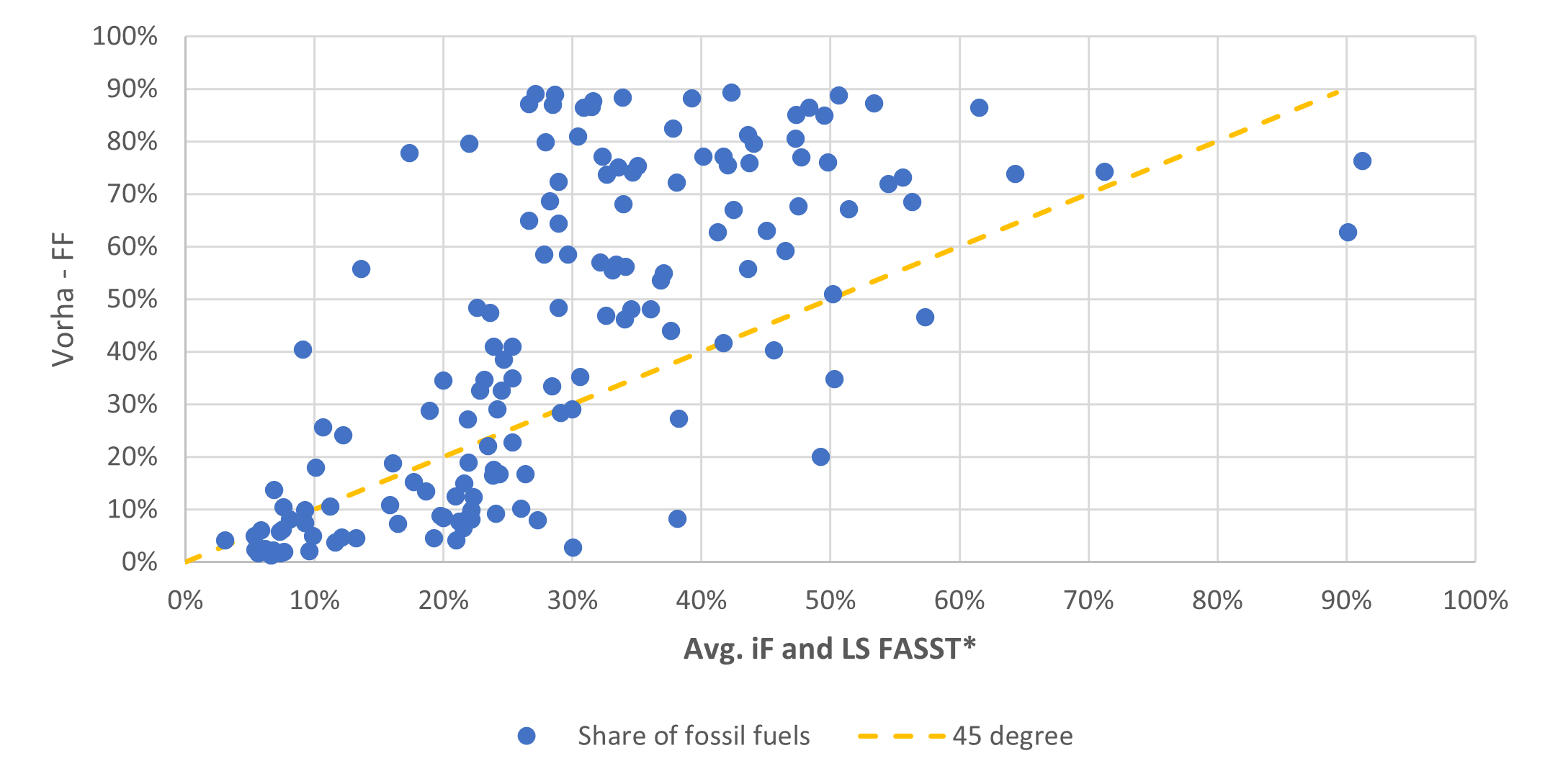
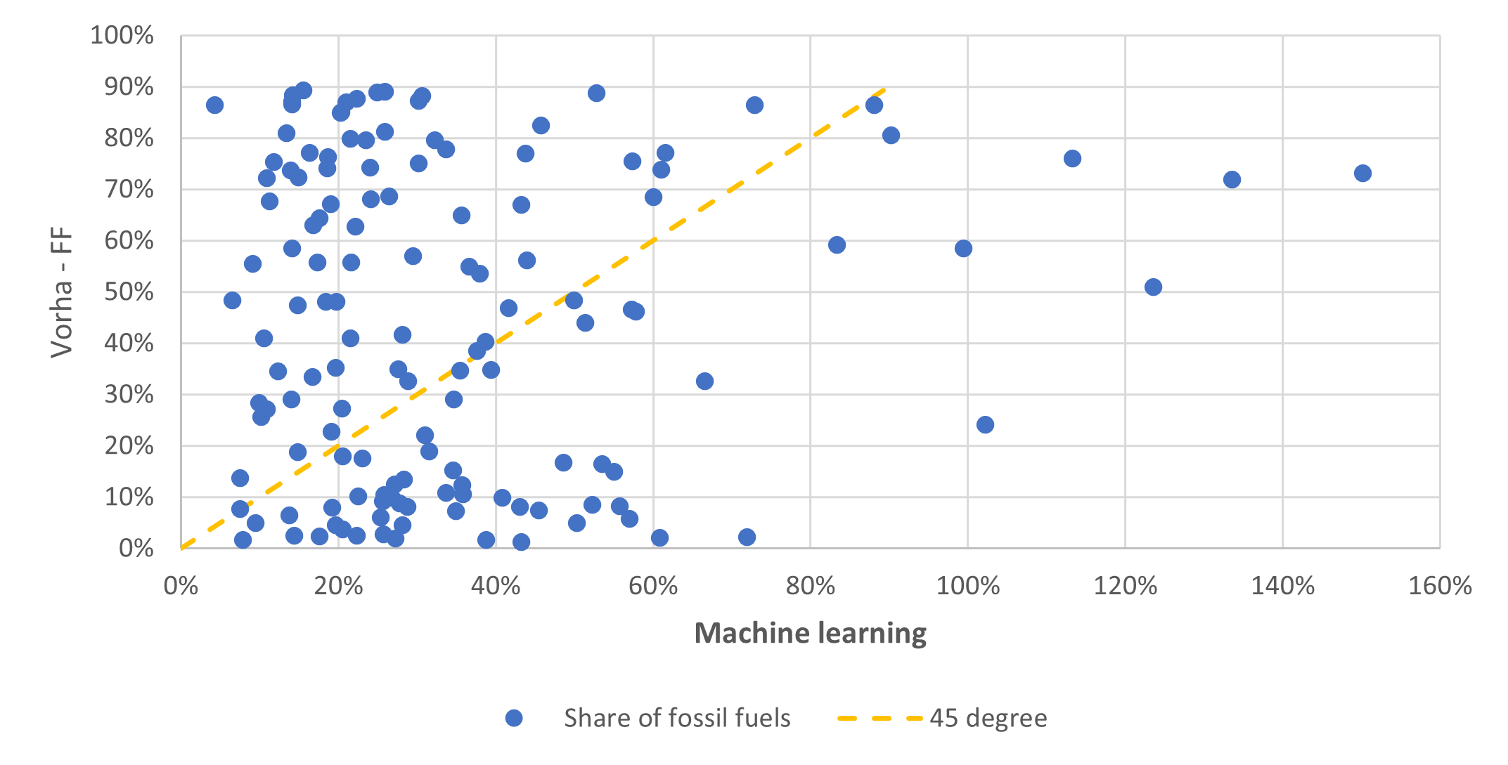
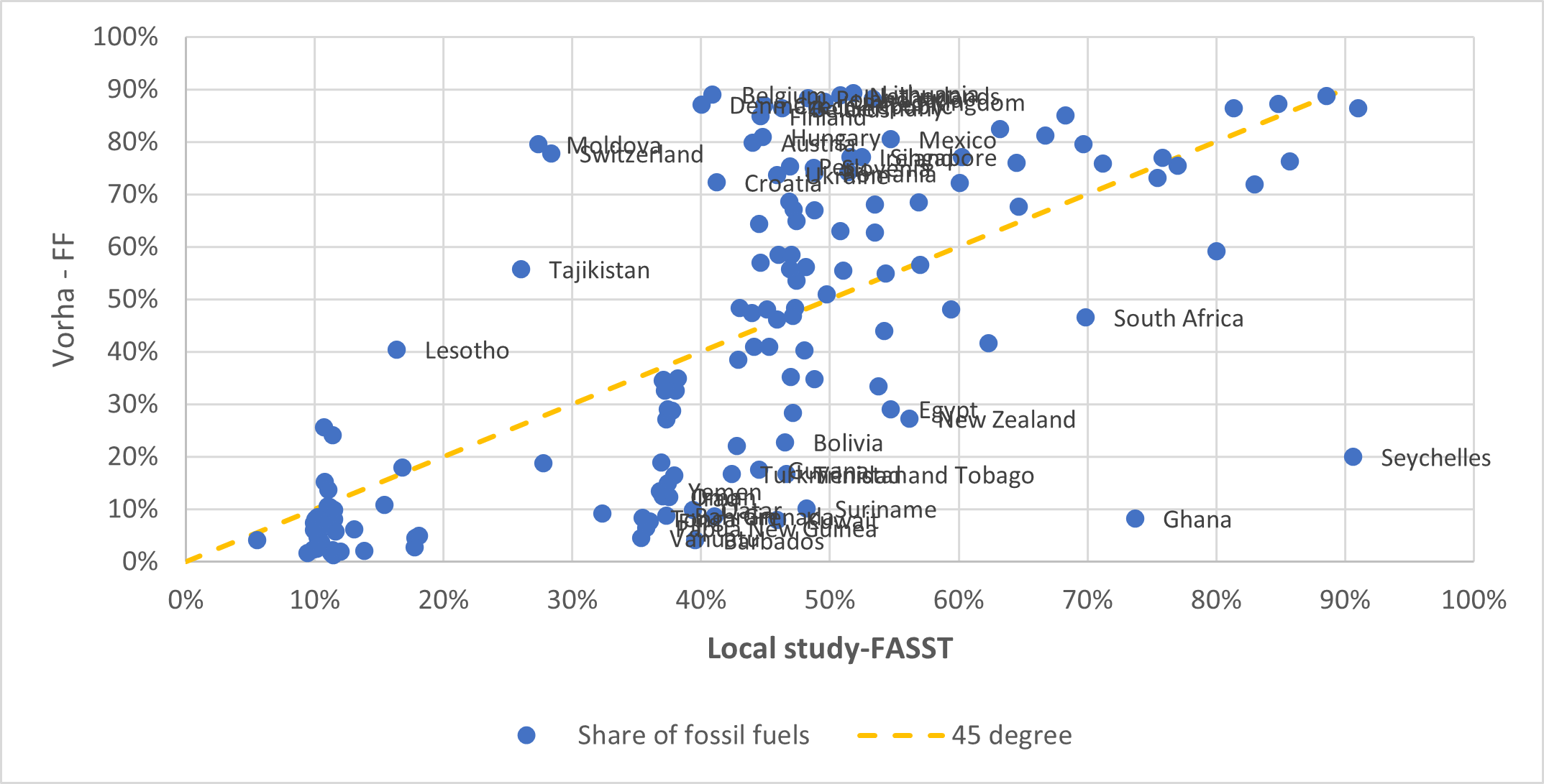
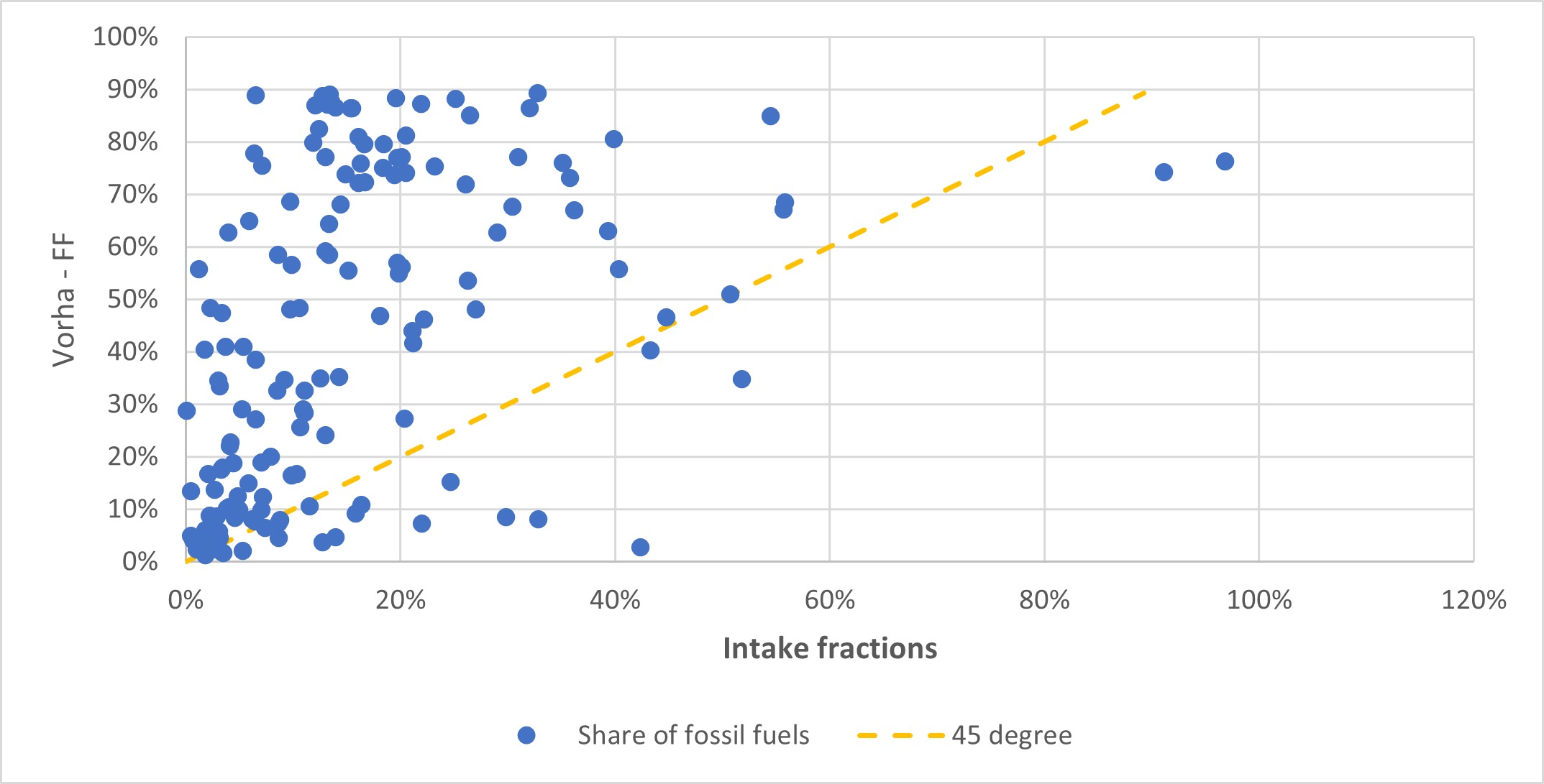
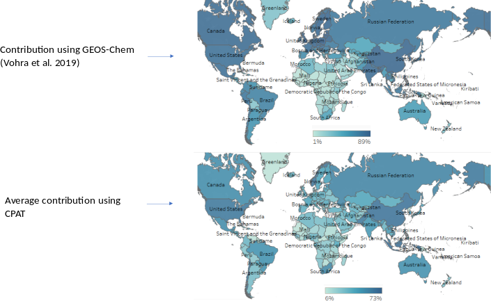
6.10.5 Comments from 2021 review and summary of changes

Below are the comments from the original review in 2021, and then our further comments in 2022. The comments in the table do not include those where reviewers were already in agreement with CPAT. Most comments and answers are a summary of the original version.

Comment	Response 2021	Response 2022
Incidence rate vs. incidence proportion The methodology document provided the definitions for key technical terms, including that for the incidence rate, which forms part of the overall method used in calculating the burden of disease. However, the definition presented in the document seems to be referring to the incidence proportion and not the rate. In epidemiological terms, there is a distinction between the two measures	Thanks for the precisions made on the definitions for incidence proportion and rate. We did use the correct measures, following the GBD study. We will correct the documentation.	The comment was incorporated into CPAT documentation.
Age-group considerations for lower respiratory tract infections (LRTI) The methodology currently considers all age groups combined for LRTI estimates and relies on the same Integrated Exposure Response (IER) function across the board for this outcome. Exposure to household air pollution almost doubles the risk for childhood pneumonia and is responsible for 45 percent of all pneumonia deaths in children less than 5 years of age. Household air pollution is also a risk for pneumonia in adults, and contributes to nearly 28 percent of all adult pneumonia-related deaths. Given implications from the application of carbon pricing, especially in relation to leakage to biomass, and households opting to use solid fuels for cooking and heating as a result, mortality estimates among those in the under 5 years old age-group is likely to increase. Therefore, stratifying LRTI cause-specific mortality by age-group to capture this specific age-group would be of extremely high relevance – even more so from an operational perspective.	We fully agree that a disaggregated analysis by age group, in buckets of five years would be the best approach, and even more disaggregated to include neonatal effects. Unfortunately, in CPAT we are working with more aggregated age groups: Under 15, 15 to 24, 25 to 64, above 65, and neonatal. We did this aggregation due to limited file size in the tool. Because of this, we cannot differentiate the effects among children under 5, but hopefully we will use a more disaggregated analysis in the CPAT version outside Excel.	As before, more detailed disaggregation is not feasible in the Excel version of the tool. But the aggregates estimate of CPAT replicate well the results obtained with more disaggregated data. In countries with high household pollution, after a carbon price we generally obtain a net reduction in health effects, despite increase household health effects.
Considering methodology applied in the Household Air Pollution Intervention Tool (HAPIT) to estimate health benefits	The team provided a comparison between HAPIT and CPAT, concluding that CPAT is based on more recent methodologies, but HAPIT does a better job differentiating exposure among women, children and men. This element could be added in a future CPAT version, developed outside Excel.	As before, regarding household pollution (not the focus of CPAT), no additional disaggregation is possible, to consider different exposure patterns among women, children and men. Regrettably we are already at the limit of Excel capabilities.
The CPAT dashboard is user-friendly and is easy to navigate. It is unclear, however, where and how to update certain parameters should the need arise (e.g. changes in IER functions, or in VSL estimates) or to allow for country-specific inputs. To this end, a more detailed user manual would be extremely valuable to have.	We hope that a few months of testing (with the team involved in each study) would give us a good idea of whether the tool can be roll out to other teams (and what type of training and support may be needed).	Now we have produced a user’s guide, that intends to guide the user about policies configuration and parameters settings. This guide corresponds to Chapter 1 of CPAT documentation.
(Emissions – concentrations – health outcomes: Of course, and the team is keenly aware of this, CPAT has to rely on simplified ways of modelling the complex relationships (such as for example using intake fractions instead of using chemical transportation modelling of relating emissions to concentrations), but for a policy tool, this in my view is certainly more than good enough. That said, I wonder if in the future we can experiment with going beyond intake fractions	Besides intake fractions, we have included other options to relate emissions and concentrations: i) TM5-FASST model, ii) Source apportionment information, in combination with TM5-FASST results and iii) Elastic Net and OLS model. We are also in the process of implementing in CPAT the results of a machine learning modeling to related emissions and concentrations, by emitting source type.	In addition to the models indicated during the previous review, we have added the following models to relate emissions to concentration: i) a machine learning methodology (simplified) and ii) Average of intake fractions and source apportionment in combination with TM5-FASST. We have also expanded the source apportionment studies available in CPAT.
I appreciate the effort made to show how CPAT’s figures correspond to IIASA’s, EDGAR’s and GBD’s, and think those are useful symmetries to show. That said, I do want to point out that this does not imply that the impact of a certain EFR on air pollution and health outcome would deliver the same results whether it’s impact is modelled with CPAT or the more complex models.	We have compared the air pollution module baseline estimates with external global sources, to make sure that we represent the baseline within the results from other more complex models. You are right that these checks do not guarantee that the policy impacts modeled in CPAT will be similar to the policy impacts obtained from other more complex models. Further checks will need to be performed in a policy/country-specific context and we have made sure that the tool allows the user to change assumptions and inputs, such the tool can be adjusted properly when needed.	We added a section of “caveats” to the documentation that includes this point.
I am currently looking at the relationships between air pollution and infant mortality, globally, as part of an ASA activity. We will be producing a concentration-response curve for this relationship, which you may choose to include into CPAT as an alternative to the GBD function.	Sure, we can add this new concentration-response curve for infant mortality in CPAT.	The paper is currently in the process of being published and the focus was on the impact of PM2.5 on increased pregnancy stunting (rather than infant mortality). This outcome can negatively affect children even after they recover from stunting. At this stage, we cannot include this effect in CPAT, but we already have children and neonatal health effects in the tool.
The pollution model includes plenty of interesting information. The direct economic link is via the reduction in labor supply and deaths related to pollution. However, there are in effect two mechanisms at play - which could be added. The first is associated with the extensive margin - i.e. the number of employed individuals not going to work due to illness. The second is related to the intensive margin - the reduction in the number of productive hours worked. This is important in a country context where affected laborers tend to be low-skilled and where laborers can be drawn from an unemployed pool and put to work immediately (the case where employing the services of an unemployed worker to replace the affected worker is costless). If this is the case, then the direct pollution effect on labor could be negligible. However, if all workers are exposed to pollution, then what matters is the intensive margin - i.e. the work effort. Reducing pollution will have an extra benefit to society - increased labor effort and more efficient means of production regardless of the substitutability of labor. At the moment the CPAT tool describes the economic benefit or reducing pollution in terms of disability adjusted life years. This is an extensive margin concept where labor rotation rates are not accounted for (i.e. the probability of drawing an unskilled worker from the unemployment pool to replace the sick worker). Accounting for these rotation rates complicates the modeling but adds another element of realism. The economic cost will no longer be associated with DALY’s multiplied by income, but with DALY’s adjusted for labor replacement effects, multiplied by incomes.	Thanks for your comments and suggestions. We agree that the “intensive margin” effect can be more relevant, due to a generalized drop in labor effort when workers are exposed to pollution. There is evidence that, besides working days lost and DALYs (both included in CPAT), productivity may decrease among workers that do attend to work. The drop in productivity has been studied in different working settings and locations of the world (see table below). We have not yet incorporated the results from the different studies into CPAT. The results of the last paper in the table (Fu, Viard, and Zhang 2017) could be implemented, if we believe that country specific results could be extrapolated and used in other countries. Moreover, there is growing evidence on cognitive effects of air pollution in adults (Allen et al. 2017; Zhang, Chen, and Zhang 2018) and neurodevelopment issues children (WHO 2018), affecting human capital formation. This implies that air pollution has both short term and long-term effects in productivity, but so far, we have not been able to incorporate them in CPAT.	As before, although the literature on productivity effects of pollution is growing, we still face the issue of location and setting specific studies, that cannot confidently be extrapolated to a global setting, for broad sectors of the economy.
When cooking fuels are exempt, the spill-over effects on consumption of various fuels particularly biomass, and the resulting health (and other development) effects should be accounted for if possible.	Thanks for this comment. Exactly, we allow the user to exempt, or rather rebate, cooking fuels in order to alleviate concerns of spill-over effects into increased biomass use. For the proportion of the consumption for which no exemption is chosen, at present we model explicit substitution into biofuels with carbon pricing (not modelled when these fuels are exempt). So, we are able to see the modelled differences in health effects between carbon price and non-carbon price (with and without exemptions).	This point was clarified during the previous review

Below is a list of the changes made in CPAT, between the 2021 review (in March) and August 2022.

Type	Description
Developments	Additional summary metrics of externalities (per unit of fuel burned), for additional fuels and sectors
	Additional indicators of externalities related to years of life lost (YLL), years lived with disabilities (YLD)
	Additional indicators of externalities differentiating for population in working age
	Inclusion of the marginal impact on global temperature, compared to emissions level of the baseline year
	New source apportionment studies were added
	New average method to relate emissions to concentrations: average of intake fractions and local-study/TM5-FASST
	New metrics about the total damage of pollution as share of GDP, using VSL and forgone output
	New option to adjust baseline year results (2019) to GBD 2019 study
	Additional VSL options
	Implementation of the results from machine learning method, for PM2.5 and ozone to relate emissions to concentrations in the different sectors.
	For household pollution, we added a projected HAP level and exposure, based in historical trends
	The relative risk functions were extended to up to 2000 ug/m3
Other changes	Emissions of local pollutants were moved to the mitigation module
	New emission factors for CO2, other GHGs and local pollutants
	Changes in graphs with results
	Dashboard results now include in their title a link to the results in the air pollution tab
	Change to a different baseline year
	Many modifications to run CPAT using the Multi Scenario tool
	Definition of default options to configure the air pollution tab
	Corrections in case modeled concentrations are above observed ones (issue arising from emissions to concentration models being calibrated with different data bases)
	Changes to more efficient (faster) formulas
	Standardization of codes (for diseases, risks, etc.)
Fixes	Many small fixes in formulas
	Runs to check errors that arises for particular countries
	Corrections to the calculation of GWP100, affected by corrections in emission for biofuels and methane.
	Correction of the average emission factors option, to calculate emissions for local air pollution health effects
	Correction of the externality of LPG. It had problems for certain emissions to concentration models.

Aleluia Reis, Lara. 2020. “Down-Scaling FASST(r) to Country Level.”

Almeida, SM, M Manousakas, E Diapouli, Z Kertesz, L Samek, E Hristova, K Šega, et al. 2020. “Ambient Particulate Matter Source Apportionment Using Receptor Modelling in European and Central Asia Urban Areas.” Environmental Pollution 266: 115199. https://doi.org/10.1016/J.ENVPOL.2020.115199.

Amann, Markus, Mike Holland, Rob Maas, T Vandyck, and B Saveyn. 2017. “Costs, Benefits and Economic Impacts of the EU Clean Air Strategy and Their Implications on Innovation and Competitiveness.” IIASA Report; International Institute for Applied Systems Analysis (IIASA): Laxenburg, Austria, 1–59. http://gains.iiasa.ac.at.ILO.

Apte, Joshua S, Emilie Bombrun, Julian D Marshall, and William W Nazaroff. 2012. “Global Intraurban Intake Fractions for Primary Air Pollutants from Vehicles and Other Distributed Sources.” Environmental Science & Technology 46 (6): 3415–23. https://doi.org/10.1021/es204021h.

Bank, World. 2022. The Global Health Cost of PM2. 5 Air Pollution: A Case for Action Beyond 2021. The World Bank.

Bennett, Deborah H, Thomas E McKone, John S Evans, William W Nazaroff, Manuele D Margni, Olivier Jolliet, and Kirk R Smith. 2002. “Defining Intake Fraction.” Environmental Science and Technology 36 (9). http://www.ncbi.nlm.nih.gov/pubmed/12026996.

Braithwaite, Isobel, Shuo Zhang, James B Kirkbride, David PJ Osborn, and Joseph F Hayes. 2019. “Air Pollution (Particulate Matter) Exposure and Associations with Depression, Anxiety, Bipolar, Psychosis and Suicide Risk: A Systematic Review and Meta-Analysis.” Environmental Health Perspectives 127 (12): 126002. https://doi.org/10.1289/EHP4595.

Byers, Logan, Johannes Friedrich, Roman Hennig, Aaron Kressig, Xinyue Li, COLIN McCormick, and Laura Malaguzzi Valeri. 2018. “A Global Database of Power Plants.” World Resources Institute 18. http://globalenergyobservatory.org.

Center for International Earth Science Information Network - CIESIN - Columbia University. 2018. “Documentation for the Gridded Population of the World, Version 4 (GPWv4), Revision 11 Data Sets.” Palisades, New York: NASA Socioeconomic Data and Applications Center (SEDAC). https://doi.org/https://doi.org/10.7927/H45Q4T5F.

Chafe, Zoë A, Michael Brauer, Zbigniew Klimont, Rita Van Dingenen, Sumi Mehta, Shilpa Rao, Keywan Riahi, Frank Dentener, and Kirk R Smith. 2014. “Household Cooking with Solid Fuels Contributes to Ambient PM2. 5 Air Pollution and the Burden of Disease.” Environmental Health Perspectives 122 (12): 1314–20. https://doi.org/10.1289/ehp.1206340.

Cropper, Maureen, Shama Gamkhar, Kabir Malik, Alexander Limonov, and Ian Partridge. 2012. “The Health Effects of Coal Electricity Generation in India.” Resources for the Future Discussion Paper, no. 12-25. https://www.rff.org/publications/working-papers/the-health-effects-of-coal-electricity-generation-in-india/.

ECLIPSE V5a Global Emission Fields - Global Emissions. 2015. “IIASA.” https://iiasa.ac.at/web/home/research/researchPrograms/air/ECLIPSEv5a.html.

European Environment Agency. 2020. “Emission Database for Global Atmospheric Research (EDGAR).” http://edgar.jrc.ec.europa.eu/.

Gaita, S. M., J. Boman, M. J. Gatari, J. B. C. Pettersson, and S. Janhäll. 2014. “Source Apportionment and Seasonal Variation of PM\(_{2.5}\) in a Sub-Saharan African City: Nairobi, Kenya.” Atmospheric Chemistry and Physics 14 (18): 9977–91. https://doi.org/10.5194/acp-14-9977-2014.

Global Burden of Disease Collaborative Network. 2018. “Global Burden of Disease Study 2017 (GBD 2017) Results.” Seattle, United States: Institute for Health Metrics and Evaluation (IHME). http://ghdx.healthdata.org/record/ihme-data/gbd-2017-life-tables-1950-2017.

Global Burden of Disease Health Financing Collaborator Network. 2019a. “Global Expected Health Spending 2017-2050.” Seattle, United States: Institute for Health Metrics and Evaluation (IHME). http://ghdx.healthdata.org/record/ihme-data/global-expected-health-spending-2017-2050.

———. 2019b. “Global Health Spending 1995-2016.” Seattle, United States: Institute for Health Metrics and Evaluation (IHME). http://ghdx.healthdata.org/record/ihme-data/global-health-spending-1995-2016.

———. 2020. “Global Burden of 87 Risk Factors in 204 Countries and Territories, 1990–2019: A Systematic Analysis for the Global Burden of Disease Study 2019.” The Lancet 396 (10258): 1223–49.

Global Energy Observatory, Google, KTH Royal Institute of Technology in Stockholm, Enipedia, World Resources Institute. 2018. “Global Power Plant Database.” Published on Resource Watch and Google Earth Engine. http://resourcewatch.org/ https://earthengine.google.com/.

Guerriero, Marta. 2019. The Labor Share of Income Around the World: Evidence from a Panel Dataset. Springer. https://www.adb.org/publications/labor-share-income-around-world-evidence-panel-dataset.

Holland, Michael. 2014. “Cost-Benefit Analysis of Final Policy Scenarios for the EU Clean Air Package.”

Humbert, Sebastien, Julian D Marshall, Shanna Shaked, Joseph V Spadaro, Yurika Nishioka, Philipp Preiss, Thomas E McKone, Arpad Horvath, and Olivier Jolliet. 2011. “Intake Fraction for Particulate Matter: Recommendations for Life Cycle Impact Assessment.” Environmental Science & Technology 45 (11): 4808–16. https://pubmed.ncbi.nlm.nih.gov/21563817/.

IEA. 2019. “Energy Prices and Taxes for OECD Countries, 4th Quarter 2019, Database Documentation.”

Inness, Antje, Melanie Ades, Anna Agustı́-Panareda, Jérôme Barré, Anna Benedictow, Anne-Marlene Blechschmidt, Juan Jose Dominguez, et al. 2019. “The CAMS Reanalysis of Atmospheric Composition.” Atmospheric Chemistry and Physics 19 (6): 3515–56.

Institute for Health Metrics and Evaluation (IHME). 2020. “GBD Results Tool.” http://ghdx.healthdata.org/gbd-results-tool.

International Road Federation. 2018. “World Road Statistics.”

IPCC and others. 2014. “Climate Change 2014: Synthesis Report. Contribution of Working Groups i, II and III to the Fifth Assessment Report of the Intergovernmental Panel on Climate Change.” Ipcc Geneva, Switzerland.

Korteland, Marisa. 2022. “Health-Related Social Costs of Air Pollution Due to Residential Heating and Cooking in the EU27 And.”

Lamancusa, Carmen, Fatema Parvez, and Kristina Wagstrom. 2017. “Spatially Resolved Intake Fraction Estimates for Primary and Secondary Particulate Matter in the United States.” Atmospheric Environment 150: 229–37.

Lelieveld, Jos, John S Evans, Mohammed Fnais, Despina Giannadaki, and Andrea Pozzer. 2015. “The Contribution of Outdoor Air Pollution Sources to Premature Mortality on a Global Scale.” Nature 525 (7569): 367–71.

Narain, Urvashi, and Chris Sall. 2016. “Methodology for Valuing the Health Impacts of Air Pollution.”

OECD. 2012. “Mortality Risk Valuation in Environment, Health and Transport Policies.” https://www.oecd-ilibrary.org/environment/mortality-risk-valuation-in-environment-health-and-transport-policies_9789264130807-en.

OECD. 2016. “The Economic Consequences of Outdoor Air Pollution.” https://doi.org/10.1787/9789264257474-en.

———. 2019. “Economic Interactions Between Climate Change and Outdoor Air Pollution.” http://www.oecd.org/officialdocuments/publicdisplaydocumentpdf/?cote=ENV/EPOC/WPIEEP(2018)3/FINAL&docLanguage=En.

———. 2020. “Health Status: Absence from Work Due to Illness.” https://stats.oecd.org/index.aspx?queryid=30123.

———. 2021a. “Inflation (CPI) (Indicator).” https://data.oecd.org/price/inflation-cpi.htm.

———. 2021b. “Level of GDP Per Capita and Productivity.” https://stats.oecd.org/Index.aspx?DataSetCode=PDB_LV.

Ostro, Bart D. 1987. “Air Pollution and Morbidity Revisited: A Specification Test.” Journal of Environmental Economics and Management 14 (1): 87–98.

Pandey, Anamika, Michael Brauer, Maureen L Cropper, Kalpana Balakrishnan, Prashant Mathur, Sagnik Dey, Burak Turkgulu, et al. 2021. “Health and Economic Impact of Air Pollution in the States of India: The Global Burden of Disease Study 2019.” The Lancet Planetary Health 5 (1): e25–38.

Parry, Ian WH, Mr Dirk Heine, Eliza Lis, and Shanjun Li. 2014. Getting Energy Prices Right: From Principle to Practice. International Monetary Fund.

Parvez, Fatema, Carmen Lamancusa, and Kristina Wagstrom. 2017. “Primary and Secondary Particulate Matter Intake Fraction from Different Height Emission Sources.” Atmospheric Environment 165: 1–11.

Preker, Alexander S, Olusoji O Adeyi, Marisa Gil Lapetra, Diane-Charlotte Simon, and Eric Keuffel. 2016. “Health Care Expenditures Associated with Pollution: Exploratory Methods and Findings.” Annals of Global Health 82 (5): 711–21.

Reid, Walter, and C Raudsepp-Hearne. 2005. “Millenium Ecosystem Assessment.”

Renna, Francesco Granella, Stefania, and Lara Aleluia Reis. 2021. “CLAQC - Country Level Air Quality Calculator.” https://datashowb.shinyapps.io/CLAQC/.

Robinson, Lisa A, James K Hammitt, Michele Cecchini, Kalipso Chalkidou, Karl Claxton, Maureen Cropper, Patrick Hoang-Vu Eozenou, et al. 2019. “Reference Case Guidelines for Benefit-Cost Analysis in Global Health and Development.”

Robinson, Lisa A, James K Hammitt, and Lucy O’Keeffe. 2019. “Valuing Mortality Risk Reductions in Global Benefit-Cost Analysis.” Journal of Benefit-Cost Analysis 10 (S1): 15–50.

Shindell, F-m Breon, D. 2013. Anthropogenic and Natural Radiative Forcing. Climate Change 2013: The Physical Science Basis.

Turner, Michelle C, Michael Jerrett, C Arden Pope III, Daniel Krewski, Susan M Gapstur, W Ryan Diver, Bernardo S Beckerman, et al. 2016. “Long-Term Ozone Exposure and Mortality in a Large Prospective Study.” American Journal of Respiratory and Critical Care Medicine 193 (10): 1134–42.

US EPA. 2013. “Regulatory Impact Analysis for the Final Revisions to the National Ambient Air Quality Standards for Particulate Matter.”

Van Dingenen, Rita, Frank Dentener, Monica Crippa, Joana Leitao, Elina Marmer, Shilpa Rao, Efisio Solazzo, and Luana Valentini. 2018. “TM5-FASST: A Global Atmospheric Source–Receptor Model for Rapid Impact Analysis of Emission Changes on Air Quality and Short-Lived Climate Pollutants.” Atmospheric Chemistry and Physics 18 (21): 16173–211. https://doi.org/10.5194/acp-18-16173-2018.

Vohra, Karn, Alina Vodonos, Joel Schwartz, Eloise A Marais, Melissa P Sulprizio, and Loretta J Mickley. 2021. “Global Mortality from Outdoor Fine Particle Pollution Generated by Fossil Fuel Combustion: Results from GEOS-Chem.” Environmental Research 195: 110754.

Wagner, F, J Borken-Kleefeld, G Kiesewetter, Z Klimont, W Schoepp, and M Amann. 2020. “Implied Emission Factors in the World Bank’s Carbon Pricing Assessment Tool (CPAT).”

Wikimedia Commons contributors. 2020. “File:DALY Disability Affected Life Year Infographic.svg.” https://commons.wikimedia.org/wiki/File:DALY_disability_affected_life_year_infographic.svg.

Woodruff, Tracey J, Jennifer D Parker, and Kenneth C Schoendorf. 2006. “Fine Particulate Matter (PM2. 5) Air Pollution and Selected Causes of Postneonatal Infant Mortality in California.” Environmental Health Perspectives 114 (5): 786–90.

World Bank. 2019a. “Air Pollution Management in North Macedonia.” World Bank.

———. 2019b. “Population Estimates and Projections.” World Bank. https://datacatalog.worldbank.org/dataset/population-estimates-and-projections.

———. 2020. Regional Note on Air Quality Management in the Western Balkans: Bosnia and Herzegovina, Kosovo, and North Macedonia. World Bank.

World Health Organization. 2015. “Database on Source Apportionment Studies for Particulate Matter in the Air (PM10 and PM<sub>2.5</Sub>).” https://www.who.int/quantifying\_ehimpacts/global/source\_apport/en/.

———. 2018. “Exposure Country Average.” Global Health Observatory Data Repository. http://apps.who.int/gho/data/node.main.152?lang=en.

World Health Organization and others. 2018. “Burden of Disease from Ambient Air Pollution for 2016 Description of Method.” WHO: Geneva, Switzerland.

Zhou, Ying, Jonathan I Levy, John S Evans, and James K Hammitt. 2006. “The Influence of Geographic Location on Population Exposure to Emissions from Power Plants Throughout China.” Environment International 32 (3): 365–73.

---

1. Air pollution contributed to 6.67 million deaths and 213 million DALYs in 2019 (Institute for Health Metrics and Evaluation)

2. Wagner, Fabian, J Borken-Kleefeld, G Kiesewetter, Z Klimont, W Schoepp, and Marcus Amann. 2020. “Implied Emission Factors in the World Bank’s Carbon Pricing Assessment Tool (CPAT).” 2020. http://dare.iiasa.ac.at/87/

3. Relative risks functions from (GBD 2019 Risk Factors Collaborators 2020)

4. For “Other energy use”, we assume an EF equal to the maximum among the EFs of the rest of the subsectors.

5. Report available in https://www.ipcc.ch/site/assets/uploads/2018/02/WG1AR5_Chapter08_FINAL.pdf, visited on April 2020.

6. POM is assumed to be equal to 1.3*OC

7. Total PM_2.5= BC + POM + Other primary PM_2.5

8. 6mDMA8h corresponds to the seasonal (six-month period with the highest mean) 8-h daily maximum concentration metric

9. Data available at http://datasets.wri.org/dataset/globalpowerplantdatabase

10. Data available in https://sedac.ciesin.columbia.edu/data/set/gpw-v4-population-count-rev11/data-download

11. Country borders from Columbia National Administrative Boundaries, v3 (2000), available in https://sedac.ciesin.columbia.edu/data/set/gpw-v3-national-admin-boundaries/data-download

12. A 30 arc-second resolution is equivalent to 1x1 km in the equator.

13. https://www.esrl.noaa.gov/psd/data/gridded/tables/precipitation.html

14. Data available in https://sedac.ciesin.columbia.edu/data/set/ma-climate-land-cover/metadata

15. Using the average generation of each plant, the estimated generation according to (World Resources Institute 2018), or a simple average among plants when no generation data is available.

16. Data available in https://datacatalog.worldbank.org/dataset/population-estimates-and-projections

17. Data available in http://apps.who.int/gho/data/node.main.152?lang=en

18. Reference from https://www.healthdata.org/terms-defined

19. Reference from https://www.healthdata.org/terms-defined

20. The new studies for China are (Yin et al. 2017) and (Li et al. 2018).

21. The age groups with different RR for Stroke and Ischemic heart disease are: 25 to 29, 30 to 34, 35 to 39, 40 to 44, 45 to 49, 50 to 54, 55 to 59, 60 to 64, 65 to 69, 70 to 74, 75 to 79, 80 to 84, 85 to 89, 90 to 94, 95+.

22. Low birthweight is been historically referred to any birthweight less than 2500 grams. TMREL $3500, 4000) g.

23. Low birthweight is a risk. The causes associated with this risk are Diarrheal diseases, Lower respiratory infections, Upper respiratory infections, Otitis media, Pneumococcal meningitis, H influenzae type B meningitis, Meningococcal meningitis, Other meningitis, Encephalitis, Neonatal preterm birth complications, Neonatal encephalopathy due to birth asphyxia and trauma, Neonatal sepsis and other neonatal infections, Haemolytic disease and other neonatal jaundice, Other neonatal disorders and Sudden infant death syndrome.

24. Preterm birth refers to newborn babies born less than 37 completed weeks of gestation. In the GBD context, “short gestation” is used to refer to all gestational ages below the gestational age TMREL. TMREL is $38, 40) weeks.

25. The WHO considers sequelae associated to different diseases or conditions.

26. Solid fuels include coal, wood, charcoal, dung, and agricultural residues.

27. Real interest rate is the lending interest rate adjusted for inflation as measured by the GDP deflator.

28. Data available in https://stats.oecd.org/index.aspx?queryid=30123

29. Data available in https://gateway.euro.who.int/en/indicators/hfa_411-2700-absenteeism-from-work-due-to-illness-days-per-employee-per-year/

30. Labor force comprises people ages 15 and older who supply labor to produce goods and services during a specified period. It includes people who are currently employed and people who are unemployed but seeking work as well as first-time jobseekers. Not everyone who works is included, however. Unpaid workers, family workers, and students are often omitted, and some countries do not count members of the armed forces. Labor force size tends to vary during the year as seasonal workers enter and leave.

31. The probability that a person dies during an interval of two ages (e.g., between birth and age 5), if the rates of all-cause mortality in a specified year of interest would remain constant into the future.

32. Data available in https://www.ilo.org/ilostat-files/Documents/Bulk_ilostat_en.html#, accessed in December 2019

33. Real interest rate is the lending interest rate adjusted for inflation as measured by the GDP deflator. The terms and conditions attached to lending rates differ by country, however, limiting their comparability.

34. Data available in https://data.worldbank.org/indicator/FR.INR.RINR, accessed in December 2019.

35. Glossary of terms here: https://dev-ilostat.pantheonsite.io/resources/concepts-and-definitions/description-earnings-and-labour-cost/